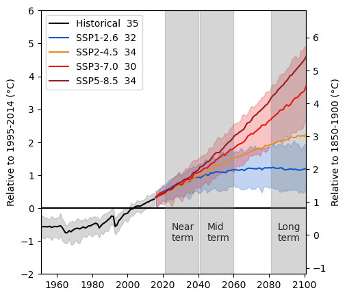
Global Surface Air Temperature changes in future scenarios

Global Surface Air Temperature changes in future scenarios#

This notebook is a reproducibility example of the IPCC-WGI AR6 Interactive Atlas products. This work is licensed under a Creative Commons Attribution 4.0 International License.

E. Cimadevilla (Santander Meteorology Group. Instituto de Física de Cantabria, CSIC-UC, Santander, Spain).

This notebook computes Global Surface Air Temperature (GSAT) changes relative to the 1995–2014 and 1850–1900 averages, according to CMIP6 climate models.

import numpy as np
import pandas as pd
import matplotlib.pyplot as plt

import xarray
import dask

dask.config.set(scheduler="processes")

<dask.config.set at 0x791c1f75d590>

Climate change indicators#

df = pd.read_csv("../../../data_inventory.csv")
subset = df.query('type == "opendap" & variable == "t" & project == "CMIP6" & frequency == "mon"')
subset

	location	type	variable	project	experiment	frequency
41	https://hub.climate4r.ifca.es/thredds/dodsC/ip...	opendap	t	CMIP6	ssp245	mon
67	https://hub.climate4r.ifca.es/thredds/dodsC/ip...	opendap	t	CMIP6	historical	mon
87	https://hub.climate4r.ifca.es/thredds/dodsC/ip...	opendap	t	CMIP6	ssp585	mon
111	https://hub.climate4r.ifca.es/thredds/dodsC/ip...	opendap	t	CMIP6	ssp370	mon
117	https://hub.climate4r.ifca.es/thredds/dodsC/ip...	opendap	t	CMIP6	ssp126	mon

hist = xarray.open_dataset(subset[subset["experiment"] == "historical"]["location"].iloc[0]).chunk(member=1, time=100)
ssp126 = xarray.open_dataset(subset[subset["experiment"] == "ssp126"]["location"].iloc[0]).chunk(member=1, time=100)
ssp245 = xarray.open_dataset(subset[subset["experiment"] == "ssp245"]["location"].iloc[0]).chunk(member=1, time=100)
ssp370 = xarray.open_dataset(subset[subset["experiment"] == "ssp370"]["location"].iloc[0]).chunk(member=1, time=100)
ssp585 = xarray.open_dataset(subset[subset["experiment"] == "ssp585"]["location"].iloc[0]).chunk(member=1, time=100)

This might give you an idea of the time required to generate the figure, in function of your working environment (remote data access or local data access).

OPeNDAP (remote data access, IFCA Hub)

CPU times: user 5min 52s, sys: 9min 8s, total: 15min
Wall time: 31min 11s

netCDF (local data access, IFCA Hub)

CPU times: user 11min 2s, sys: 2min 58s, total: 14min
Wall time: 14min 46s

%%time

weights = np.cos(np.deg2rad(hist["lat"]))
mean_hist_1995_2014 = hist["t"].sel(time=slice("19950101", "20141231")).weighted(weights).mean(["time", "lat", "lon"]).compute(num_workers=4)
mean_hist_1850_1900 = hist["t"].sel(time=slice("18500101", "19001231")).weighted(weights).mean(["time", "lat", "lon"]).compute(num_workers=4)

mean_hist = hist["t"].sel(time=slice("19500101", None)).weighted(weights).mean(["member", "lat", "lon"]).compute(num_workers=4)
mean_ssp126 = ssp126["t"].weighted(weights).mean(["member", "lat", "lon"]).compute(num_workers=4)
mean_ssp245 = ssp245["t"].weighted(weights).mean(["member", "lat", "lon"]).compute(num_workers=4)
mean_ssp370 = ssp370["t"].weighted(weights).mean(["member", "lat", "lon"]).compute(num_workers=4)
mean_ssp585 = ssp585["t"].weighted(weights).mean(["member", "lat", "lon"]).compute(num_workers=4)

mean_spatial_hist = hist["t"].sel(time=slice("19500101", None)).weighted(weights).mean(["lat", "lon"]).compute(num_workers=4)
mean_spatial_ssp126 = ssp126["t"].weighted(weights).mean(["lat", "lon"]).compute(num_workers=4)
mean_spatial_ssp245 = ssp245["t"].weighted(weights).mean(["lat", "lon"]).compute(num_workers=4)
mean_spatial_ssp370 = ssp370["t"].weighted(weights).mean(["lat", "lon"]).compute(num_workers=4)
mean_spatial_ssp585 = ssp585["t"].weighted(weights).mean(["lat", "lon"]).compute(num_workers=4)

mean_hist_1995_2014_YE = (mean_hist - mean_hist_1995_2014).resample(time="YE").mean()
mean_ssp126_1995_2014_YE = (mean_ssp126 - mean_hist_1995_2014).resample(time="YE").mean()
mean_ssp245_1995_2014_YE = (mean_ssp245 - mean_hist_1995_2014).resample(time="YE").mean()
mean_ssp370_1995_2014_YE = (mean_ssp370 - mean_hist_1995_2014).resample(time="YE").mean()
mean_ssp585_1995_2014_YE = (mean_ssp585 - mean_hist_1995_2014).resample(time="YE").mean()

mean_hist_1850_1900_YE = (mean_hist - mean_hist_1850_1900).resample(time="YE").mean()
mean_ssp126_1850_1900_YE = (mean_ssp126 - mean_hist_1850_1900).resample(time="YE").mean()
mean_ssp245_1850_1900_YE = (mean_ssp245 - mean_hist_1850_1900).resample(time="YE").mean()
mean_ssp370_1850_1900_YE = (mean_ssp370 - mean_hist_1850_1900).resample(time="YE").mean()
mean_ssp585_1850_1900_YE = (mean_ssp585 - mean_hist_1850_1900).resample(time="YE").mean()

q_hist_1995_2014_YE = (mean_spatial_hist - mean_hist_1995_2014).resample(time="YE").mean().quantile([.05, .95], dim=["member"])
q_ssp126_1995_2014_YE = (mean_spatial_ssp126 - mean_hist_1995_2014).resample(time="YE").mean().quantile([.05, .95], dim=["member"])
q_ssp245_1995_2014_YE = (mean_spatial_ssp245 - mean_hist_1995_2014).resample(time="YE").mean().quantile([.05, .95], dim=["member"])
q_ssp370_1995_2014_YE = (mean_spatial_ssp370 - mean_hist_1995_2014).resample(time="YE").mean().quantile([.05, .95], dim=["member"])
q_ssp585_1995_2014_YE = (mean_spatial_ssp585 - mean_hist_1995_2014).resample(time="YE").mean().quantile([.05, .95], dim=["member"])

CPU times: user 5min 52s, sys: 9min 8s, total: 15min
Wall time: 31min 11s

Plot the results. Note that this figure aims to reproduce the same one from the IPCC AR6 Chapter 4, Figure 4.2 but with different model members.

fig, ax = plt.subplots(figsize=(5,5))

ytop = 6

ax.fill_between(q_hist_1995_2014_YE.time,
                q_hist_1995_2014_YE.sel(quantile=.05),
                q_hist_1995_2014_YE.sel(quantile=.95),
                color="#616161", alpha=0.25)
ax.fill_between(q_ssp126_1995_2014_YE.time,
                q_ssp126_1995_2014_YE.sel(quantile=.05),
                q_ssp126_1995_2014_YE.sel(quantile=.95),
                color="#0e57cc", alpha=0.25)
ax.fill_between(q_ssp370_1995_2014_YE.time,
                q_ssp370_1995_2014_YE.sel(quantile=.05),
                q_ssp370_1995_2014_YE.sel(quantile=.95),
                color="#e81515", alpha=0.25)
ax.set_ylim([-2, ytop])
ax.set_ylabel("Relative to 1995-2014 (°C)")
ax.axhline(y=0, color="black")
ax.text(np.datetime64('2024-12-31T00:00:00.000000000'), -1, "Near\nterm")
ax.text(np.datetime64('2044-12-31T00:00:00.000000000'), -1, "Mid\nterm")
ax.text(np.datetime64('2084-12-31T00:00:00.000000000'), -1, "Long\nterm")

ax2 = ax.twinx()
ax2.plot(mean_hist_1850_1900_YE.time, mean_hist_1850_1900_YE.mean("member"), color="#010101", label=f"Historical  {len(hist['member'])}")
ax2.plot(mean_ssp126_1850_1900_YE.time, mean_ssp126_1850_1900_YE.mean("member"), color="#0e57cc", label=f"SSP1-2.6  {len(ssp126['member'])}")
ax2.plot(mean_ssp245_1850_1900_YE.time, mean_ssp245_1850_1900_YE.mean("member"), color="#e68d26", label=f"SSP2-4.5  {len(ssp245['member'])}")
ax2.plot(mean_ssp370_1850_1900_YE.time, mean_ssp370_1850_1900_YE.mean("member"), color="#e81515", label=f"SSP3-7.0  {len(ssp370['member'])}")
ax2.plot(mean_ssp585_1850_1900_YE.time, mean_ssp585_1850_1900_YE.mean("member"), color="#9b1a22", label=f"SSP5-8.5  {len(ssp585['member'])}")
ax2.set_ylabel("Relative to 1850-1900 (°C)")
ax2.set_ylim(bottom=-2+.82, top=ytop+.82)

ax2.fill_between(
    mean_ssp126_1995_2014_YE["time"].sel(time=slice("20200101", "20400101")),
    -2+.82, ytop+.82, alpha=.33, color="grey")
ax2.fill_between(
    mean_ssp126_1995_2014_YE["time"].sel(time=slice("20400101", "20600101")),
    -2+.82, ytop+.82, alpha=.33, color="grey")
ax2.fill_between(
    mean_ssp126_1995_2014_YE["time"].sel(time=slice("20800101", None)),
    -2+.82, ytop+.82, alpha=.33, color="grey")

ax.margins(0)
ax2.margins(0)
ax2.legend()

plt.savefig("t_CMIP6_scenarios.svg")

../_images/30100dc93169b843d38ba3d1591be832092dd597716998aab9f5d5056cdc6a45.png

Global Surface Air Temperature changes in future scenarios

Contents

Global Surface Air Temperature changes in future scenarios#

Climate change indicators#