Projected climate change signals and uncertainty under global warming levels#
This notebook is a reproducibility example of the IPCC-WGI AR6 Interactive Atlas products. This work is licensed under a Creative Commons Attribution 4.0 International License.

E. Cimadevilla and M. Iturbide (Santander Meteorology Group. Instituto de Física de Cantabria, CSIC-UC, Santander, Spain).
This notebook is an example of the calculation and visualization of the IPCC-WGI AR6 uncertainty methods (simple and advanced) for projected delta changes. Please refer to the AR6 WGI Cross-Chapter Box Atlas 1 (Gutiérrez et al., 2021) for more information. We also introduce the Global Warming Level dimension for the analysis of the climate change signal.
See also hatching-uncertainty_R.ipynb at the IPCC-WGI/Atlas GitHub repository (also available in the hub: shared/repositories/IPCC-WGI-Atlas/notebooks).
This notebook works with the data available in this Hub, this is the dataset underlying the IPCC-WGI AR6 Interactive Atlas, originally published at DIGITAL.CSIC for the long-term archival, and also available through the Copernicus Data Store (CDS). Open the Getting_started.ipynb for a quick description of the available data.
Contents in this notebook#
Libraries
The Global Warming Level analysis dimension
Data loading for the different GWLs
Data loading for the historical reference
Uncertainty calculation and representation
1. Libraries#
import re
import math

import xarray
import numpy as np
import pandas as pd
import cartopy.crs as ccrs
import matplotlib.pyplot as plt
import requests
2. The Global Warming Level analysis dimension#
Instead of calculating climate change anomalies for a fixed period, we will calculate the anomaly for a given level of global warming (GWL). To do so, we need the information on the time windows where the global surface temperature reaches the different levels of warming. This information is available at the IPCC-WGI/Atlas GitHub repository.
url = "https://github.com/SantanderMetGroup/ATLAS/raw/refs/heads/main/warming-levels/CMIP6_Atlas_WarmingLevels.csv"
gwls_file = url.split("/")[-1]
with open(gwls_file, "w") as f:
    response = requests.get(url)
    response.raise_for_status()
    f.write(response.text)
gwls = pd.read_csv(gwls_file)
gwls.head()
| model_run | 1.5_ssp126 | 2_ssp126 | 3_ssp126 | 4_ssp126 | 1.5_ssp245 | 2_ssp245 | 3_ssp245 | 4_ssp245 | 1.5_ssp370 | 2_ssp370 | 3_ssp370 | 4_ssp370 | 1.5_ssp585 | 2_ssp585 | 3_ssp585 | 4_ssp585 | |
|---|---|---|---|---|---|---|---|---|---|---|---|---|---|---|---|---|---|
| 0 | ACCESS-CM2_r1i1p1f1 | 2027.0 | 2042.0 | NaN | NaN | 2028 | 2040 | 2070.0 | NaN | 2027 | 2039 | 2062.0 | 2082.0 | 2025 | 2038 | 2055 | 2071.0 |
| 1 | ACCESS-ESM1-5_r1i1p1f1 | 2030.0 | 2072.0 | NaN | NaN | 2029 | 2045 | NaN | NaN | 2033 | 2048 | 2069.0 | NaN | 2027 | 2039 | 2060 | 2078.0 |
| 2 | AWI-CM-1-1-MR_r1i1p1f1 | 2022.0 | 2050.0 | NaN | NaN | 2020 | 2039 | NaN | NaN | 2021 | 2037 | 2064.0 | NaN | 2019 | 2036 | 2059 | 2079.0 |
| 3 | BCC-CSM2-MR_r1i1p1f1 | 2041.0 | NaN | NaN | NaN | 2035 | 2057 | NaN | NaN | 2032 | 2046 | 2074.0 | NaN | 2031 | 2043 | 2065 | NaN |
| 4 | CAMS-CSM1-0_r2i1p1f1 | NaN | NaN | NaN | NaN | 2055 | 2088 | NaN | NaN | 2046 | 2065 | NaN | NaN | 2047 | 2064 | 2088 | NaN |
Note that we have pointed to the CMIP6_Atlas_WarmingLevels.csv file, as we are going to work with CMIP6 data. In this example, we will focus on the +3ºC GWL. We will consider the ssp585 scenario, however, any other scenario can be considered, as the anomalies do not vary significantly across scenarios when the GWL dimension is analyzed.
gwls3 = gwls[["model_run", "3_ssp585"]]
gwls3.head()
| model_run | 3_ssp585 | |
|---|---|---|
| 0 | ACCESS-CM2_r1i1p1f1 | 2055 |
| 1 | ACCESS-ESM1-5_r1i1p1f1 | 2060 |
| 2 | AWI-CM-1-1-MR_r1i1p1f1 | 2059 |
| 3 | BCC-CSM2-MR_r1i1p1f1 | 2065 |
| 4 | CAMS-CSM1-0_r2i1p1f1 | 2088 |
Object gwl3 is a data frame containing the central year in a time window of 20 years where the +3ºC GWL is reached for each model (Find more information in the IPCC-WGI/Atlas repository).
3. Data loading for the different GWLs#
df = pd.read_csv("../../../data_inventory.csv")
subset = df.query('type == "opendap" & variable == "pr" & project == "CMIP6" & experiment == "ssp585" & frequency == "mon"')
location = subset["location"].iloc[0]
location
'https://hub.climate4r.ifca.es/thredds/dodsC/ipcc/ar6/atlas/ia-monthly/CMIP6/ssp585/pr_CMIP6_ssp585_mon_201501-210012.nc'
cmip6_ssp585 = xarray.open_dataset(location)
cmip6_ssp585["member"] = cmip6_ssp585["member"].astype(str)  # due to OPeNDAP reading as bytes
cmip6_ssp585["member"] = [re.sub(r"[^_]+_", "", x, count=1) for x in cmip6_ssp585["member"].values]  # due to different values

lats, lons = slice(35, 72), slice(-11, 35)

# common members
members = [x for x in cmip6_ssp585["member"].values if x in gwls["model_run"].values]
gwls3_ssp585 = gwls3[gwls3["model_run"].isin(members)]
cmip6_ssp585 = cmip6_ssp585.sel(
    member=members,
    lat=lats,
    lon=lons,
    time=cmip6_ssp585.time.dt.month.isin([12,1,2]))

cmip6_ssp585
<xarray.Dataset> Size: 58MB
Dimensions:    (member: 33, time: 258, lat: 37, lon: 46, bnds: 2)
Coordinates:
  * member     (member) <U24 3kB 'ACCESS-CM2_r1i1p1f1' ... 'UKESM1-0-LL_r1i1p...
  * time       (time) datetime64[ns] 2kB 2015-01-01 2015-02-01 ... 2100-12-01
  * lat        (lat) float64 296B 35.5 36.5 37.5 38.5 ... 68.5 69.5 70.5 71.5
  * lon        (lon) float64 368B -10.5 -9.5 -8.5 -7.5 ... 31.5 32.5 33.5 34.5
Dimensions without coordinates: bnds
Data variables:
    time_bnds  (time, bnds) datetime64[ns] 4kB ...
    lat_bnds   (lat, bnds) float64 592B ...
    lon_bnds   (lon, bnds) float64 736B ...
    crs        int32 4B ...
    pr         (member, time, lat, lon) float32 58MB ...
Attributes:
    Conventions:               CF-1.9 ACDD-1.3
    summary:                   IPCC-WGI AR6 Interactive Atlas dataset: Monthl...
    keywords:                  CMIP5, CMIP6, CORDEX, IPCC, Interactive Atlas
    institution:               Instituto de Fisica de Cantabria (IFCA, CSIC-U...
    license:                   CC-BY 4.0, https://creativecommons.org/license...
    references:                https://doi.org/10.1017/9781009157896.021 http...
    standard_name_vocabulary:  CF Standard Name Table (Version 79, 2022-03-19)
    experiment_id:             ssp585
    source:                    CMIP6
    frequency:                 mon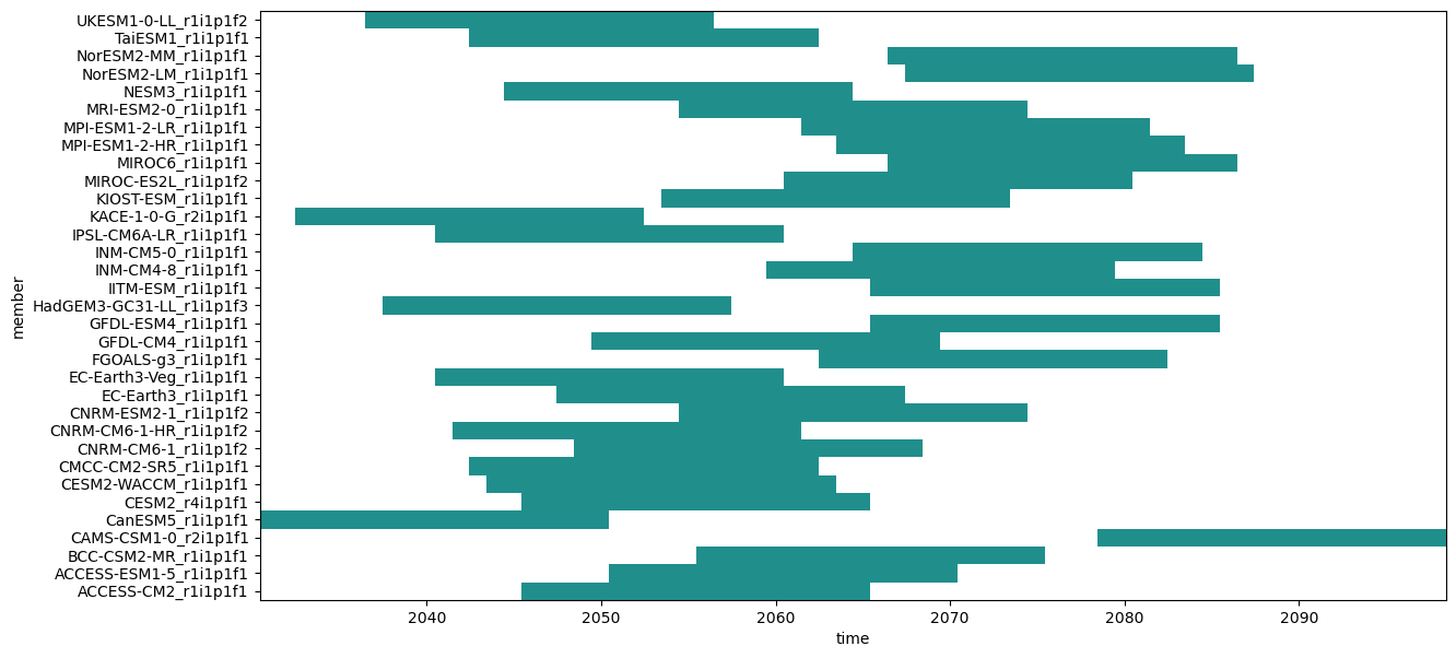
variable_id: prcmip6_ssp585 = xarray.concat(
[cmip6_ssp585.sel(
member=model_run,
time=slice(f"{year-10}1201", f"{year+10}0201"))
for model_run, year in gwls3_ssp585.values
if year != 9999],
"member")
cmip6_ssp585
<xarray.Dataset> Size: 46MB
Dimensions:    (member: 33, time: 204, bnds: 2, lat: 37, lon: 46)
Coordinates:
  * time       (time) datetime64[ns] 2kB 2030-12-01 2031-01-01 ... 2098-02-01
  * lat        (lat) float64 296B 35.5 36.5 37.5 38.5 ... 68.5 69.5 70.5 71.5
  * lon        (lon) float64 368B -10.5 -9.5 -8.5 -7.5 ... 31.5 32.5 33.5 34.5
  * member     (member) <U24 3kB 'ACCESS-CM2_r1i1p1f1' ... 'UKESM1-0-LL_r1i1p...
Dimensions without coordinates: bnds
Data variables:
    time_bnds  (member, time, bnds) datetime64[ns] 108kB NaT NaT NaT ... NaT NaT
    lat_bnds   (member, lat, bnds) float64 20kB 35.0 36.0 36.0 ... 71.0 72.0
    lon_bnds   (member, lon, bnds) float64 24kB -11.0 -10.0 -10.0 ... 34.0 35.0
    crs        (member) int32 132B -2147483647 -2147483647 ... -2147483647
    pr         (member, time, lat, lon) float32 46MB nan nan nan ... nan nan nan
Attributes:
    Conventions:               CF-1.9 ACDD-1.3
    summary:                   IPCC-WGI AR6 Interactive Atlas dataset: Monthl...
    keywords:                  CMIP5, CMIP6, CORDEX, IPCC, Interactive Atlas
    institution:               Instituto de Fisica de Cantabria (IFCA, CSIC-U...
    license:                   CC-BY 4.0, https://creativecommons.org/license...
    references:                https://doi.org/10.1017/9781009157896.021 http...
    standard_name_vocabulary:  CF Standard Name Table (Version 79, 2022-03-19)
    experiment_id:             ssp585
    source:                    CMIP6
    frequency:                 mon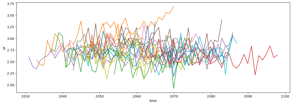
variable_id: prqmean = cmip6_ssp585.mean(["lat", "lon"]).resample(time="QS-DEC").mean()
plot = qmean["pr"].sel(time=qmean["pr"].time.dt.month==12).plot.line(x="time", add_legend=False, figsize=(15, 5))
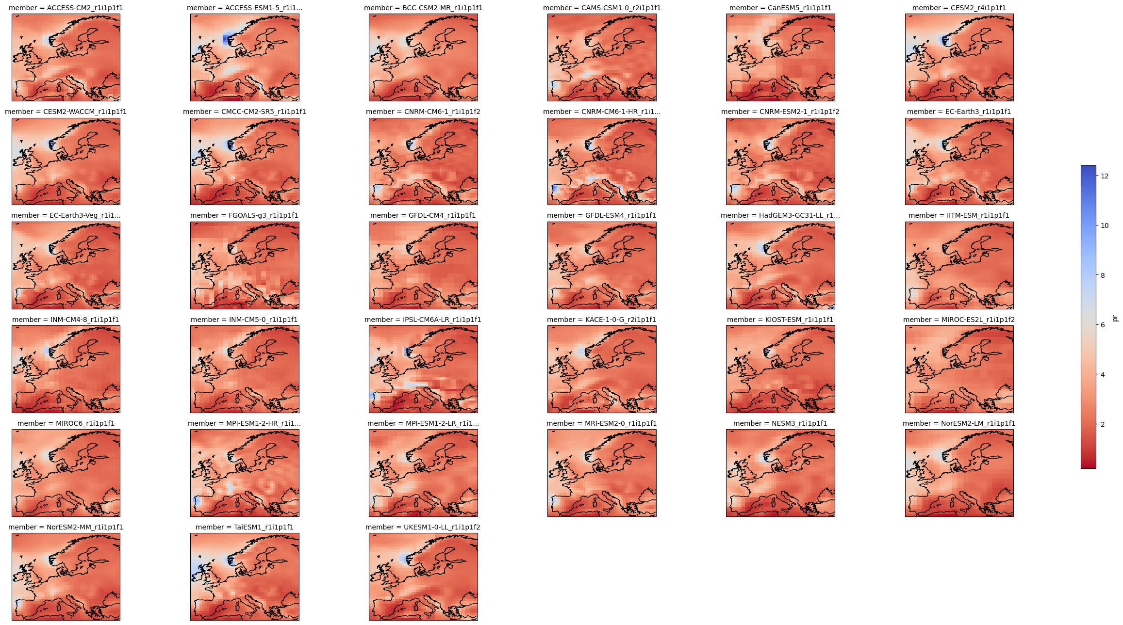
plot = cmip6_ssp585["pr"].mean("time").plot(
    x="lon", y="lat", col="member", col_wrap=6,
    figsize=(28,13),
    add_colorbar=True,
    cmap="coolwarm_r",
    cbar_kwargs={"shrink": .5},
    subplot_kws=dict(projection=ccrs.PlateCarree(central_longitude=0)),
    transform=ccrs.PlateCarree())

for ax in plot.axs.flatten():
    ax.coastlines()
    ax.set_extent((lons.start, lons.stop, lats.start, lats.stop), ccrs.PlateCarree())
4. Data loading for the historical reference#
To get the climate change signal, we first need to load data from the historical scenario. As mentioned above, we are considering the pre-industrial period. In this case, the reference period is common to all models, therefore the process becomes simpler; all models are loaded at once into a single grid object and we do not need to set a loop.
df = pd.read_csv("../../data_inventory.csv")
subset = df.query('type == "opendap" & variable == "pr" & project == "CMIP6" & experiment == "historical" & frequency == "mon"')
location = subset["location"].iloc[0]
location
'https://hub.climate4r.ifca.es/thredds/dodsC/ipcc/ar6/atlas/ia-monthly/CMIP6/historical/pr_CMIP6_historical_mon_185001-201412.nc'
cmip6_hist = xarray.open_dataset(location).sel(
    lat=lats,
    lon=lons,
    time=slice("18501201", "19000201"))
cmip6_hist["member"] = cmip6_hist["member"].astype(str)  # due to OPeNDAP reading as bytes
cmip6_hist["member"] = [re.sub(r"[^_]+_", "", x, count=1) for x in cmip6_hist["member"].values]  # due to different values

# common members
members = [x for x in cmip6_ssp585["member"].values if x in cmip6_hist["member"].values]
cmip6_hist = cmip6_hist.sel(
    member=members,
    time=cmip6_hist.time.dt.month.isin([12,1,2]))

cmip6_hist
<xarray.Dataset> Size: 34MB
Dimensions:    (member: 33, time: 150, lat: 37, lon: 46, bnds: 2)
Coordinates:
  * member     (member) <U25 3kB 'ACCESS-CM2_r1i1p1f1' ... 'UKESM1-0-LL_r1i1p...
  * time       (time) datetime64[ns] 1kB 1850-12-01 1851-01-01 ... 1900-02-01
  * lat        (lat) float64 296B 35.5 36.5 37.5 38.5 ... 68.5 69.5 70.5 71.5
  * lon        (lon) float64 368B -10.5 -9.5 -8.5 -7.5 ... 31.5 32.5 33.5 34.5
Dimensions without coordinates: bnds
Data variables:
    time_bnds  (time, bnds) datetime64[ns] 2kB ...
    lat_bnds   (lat, bnds) float64 592B ...
    lon_bnds   (lon, bnds) float64 736B ...
    crs        int32 4B ...
    pr         (member, time, lat, lon) float32 34MB ...
Attributes:
    Conventions:               CF-1.9 ACDD-1.3
    summary:                   IPCC-WGI AR6 Interactive Atlas dataset: Monthl...
    keywords:                  CMIP5, CMIP6, CORDEX, IPCC, Interactive Atlas
    institution:               Instituto de Fisica de Cantabria (IFCA, CSIC-U...
    license:                   CC-BY 4.0, https://creativecommons.org/license...
    references:                https://doi.org/10.1017/9781009157896.021 http...
    standard_name_vocabulary:  CF Standard Name Table (Version 79, 2022-03-19)
    experiment_id:             historical
    source:                    CMIP6
    frequency:                 mon
variable_id: prIt is always a good practice to make sure that the members in both grids are identical:
print(f'Are all members identical? {(cmip6_hist["member"] == cmip6_ssp585["member"]).all().item()}')
Are all members identical? True
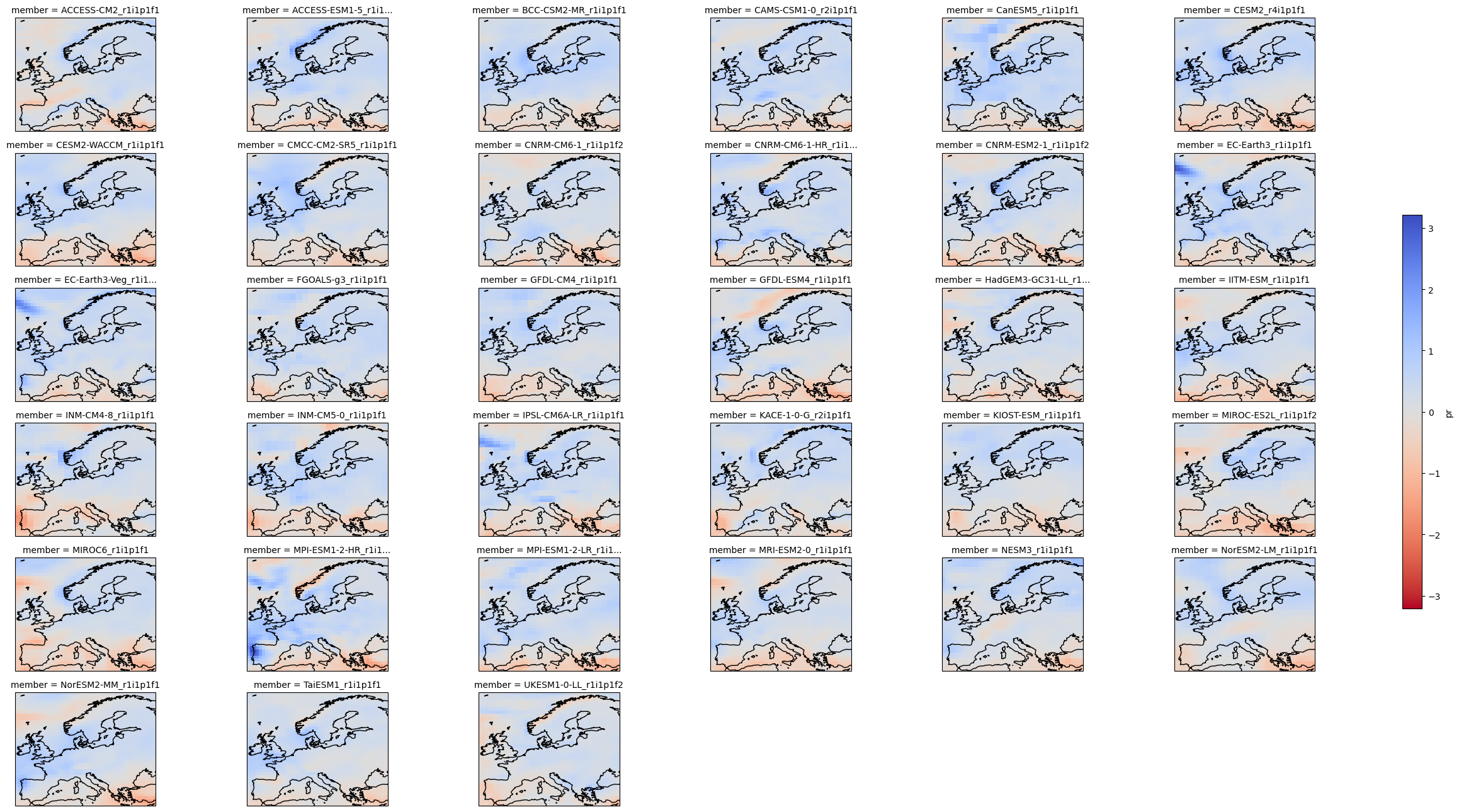
Now we can calculate the anomaly by computing the difference between both climatologies:
%%time

delta = cmip6_ssp585["pr"].mean("time") - cmip6_hist["pr"].mean("time")
CPU times: user 5.78 s, sys: 1.43 s, total: 7.22 s
Wall time: 2min 7s
plot = delta.plot(
    x="lon", y="lat", col="member", col_wrap=6,
    figsize=(28,13),
    add_colorbar=True,
    cmap="coolwarm_r",
    cbar_kwargs={"shrink": .5},
    subplot_kws=dict(projection=ccrs.PlateCarree(central_longitude=0)),
    transform=ccrs.PlateCarree())

for ax in plot.axs.flatten():
    ax.coastlines()
    ax.set_extent((lons.start, lons.stop, lats.start, lats.stop), ccrs.PlateCarree())

plot.fig.savefig("pr-delta.svg")
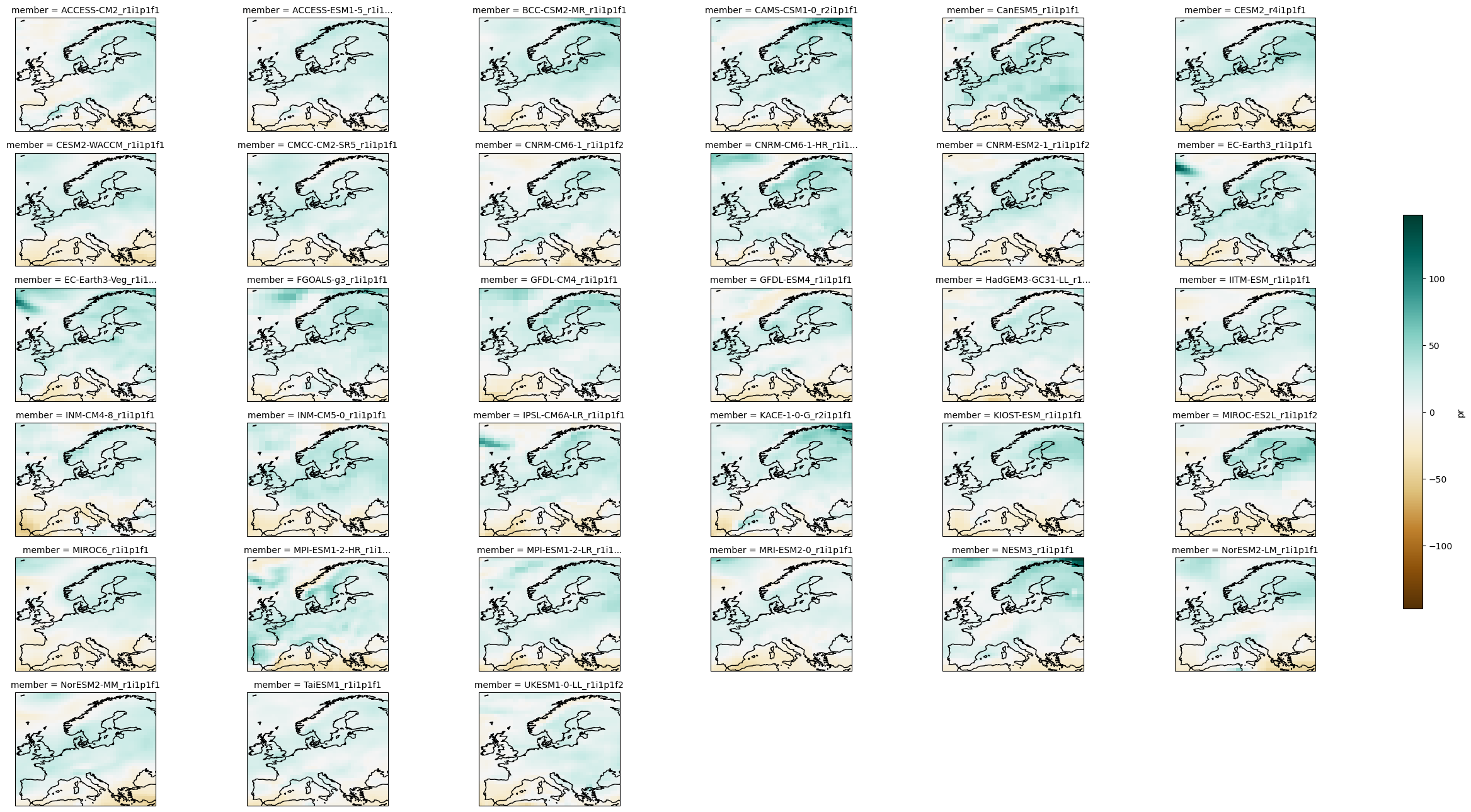
We can calculate the relative anomaly the same way:
delta_rel = (delta / cmip6_hist["pr"].mean("time")) * 100
plot = delta_rel.plot(
    x="lon", y="lat", col="member", col_wrap=6,
    figsize=(28,13),
    add_colorbar=True,
    cmap="BrBG",
    cbar_kwargs={"shrink": .5},
    subplot_kws=dict(projection=ccrs.PlateCarree(central_longitude=0)),
    transform=ccrs.PlateCarree())

for ax in plot.axs.flatten():
    ax.coastlines()
    ax.set_extent((lons.start, lons.stop, lats.start, lats.stop), ccrs.PlateCarree())
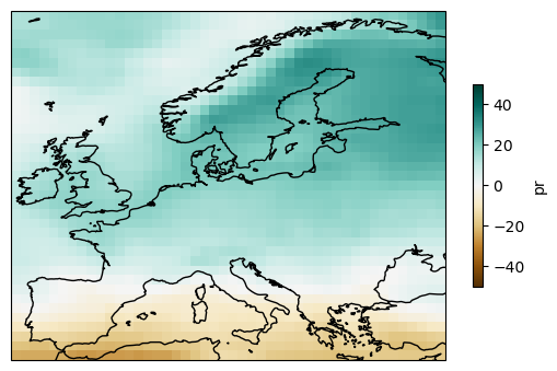
To calculate the multi-model mean, use function aggregateGrid.
ens_mean = delta_rel.mean("member")

plot = ens_mean.plot(
    add_colorbar=True,
    cmap="BrBG",
    cbar_kwargs={"shrink": .5},
    vmin=-50, vmax=50,
    subplot_kws=dict(projection=ccrs.PlateCarree(central_longitude=0)),
    transform=ccrs.PlateCarree())

plot.axes.coastlines()
<cartopy.mpl.feature_artist.FeatureArtist at 0x7adaab125e10>
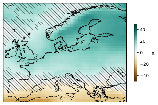
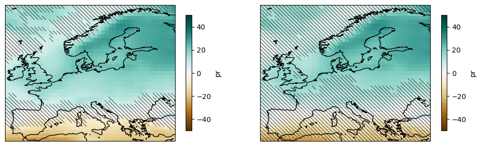
5. Uncertainty calculation and representation#
climate4R implements the “simple” and “advanced” methods for the uncertainty characterization defined in the IPCC Sixth Assessment report. The function to apply is computeUncertainty. Please refer to the AR6 WGI Cross-Chapter Box Atlas 1 (Gutiérrez et al., 2021) for more information.
def model_agreement(da, axis, th = 80):
    nmembers, nlat, nlon = da.shape
    mask = np.array([
        (da[:,i,j] > 0).sum() > int(nmembers * th / 100)
        if da[:,i,j].mean() > 0
        else (da[:,i,j] < 0).sum() > int(nmembers * th / 100)
        for i in range(nlat)
        for j in range(nlon)]).reshape((nlat,nlon))

    return mask

def hatching(plot, mask, data):
    rows, cols = mask.shape
    for i in range(rows):
        for j in range(cols):
            lat, lon = data["lat"][i].item(), data["lon"][j].item()
            if mask[i,j]:
                plot.axes.plot([lon-.5,lon+.5],[lat+.5,lat-.5],'-',c="black", linewidth=.5)
mask_simple = delta.reduce(model_agreement, "member")

plot = ens_mean.plot(
    add_colorbar=True,
    cmap="BrBG",
    cbar_kwargs={"shrink": .5},
    vmin=-50, vmax=50,
    subplot_kws=dict(projection=ccrs.PlateCarree(central_longitude=0)),
    transform=ccrs.PlateCarree())

hatching(plot, ~mask_simple, ens_mean)

plot.axes.coastlines()

plt.savefig("uncer-europe.svg", bbox_inches="tight")
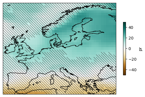
Now we compute the “advanced” method:
def advanced_method(historical, delta):
    vth = historical.reduce(
        lambda da, axis: ((math.sqrt(2) * 1.645 * np.std(da, axis=axis, ddof=1)) / math.sqrt(20)),
        "time")
    anom_abs = np.abs(delta)
    sig = anom_abs - vth
    si = xarray.where(sig > 0, 1, 0)
    uncer3 = delta.reduce(model_agreement, "member", th=80)
    uncer1 = si.reduce(
        lambda da, axis, nmembers, th: (da.sum(axis)/nmembers)*100 > th,
        "member",
        nmembers=si["member"].size,
        th=66)
    uncer2 = si.reduce(
        lambda da, axis, nmembers, th: (da.sum(axis)/nmembers)*100 < th,
        "member",
        nmembers=si["member"].size,
        th=66)
    uncer23 = (uncer2.astype(int) + uncer3.astype(int)) > 0
    uncer_a_aux1 = ((uncer1.astype(int) - 1) * -1).values
    uncer_a_aux2 = ((uncer23.astype(int) - 1) * -1).values
    uncer_a_aux2[uncer_a_aux2 == 1] = 2
    uncer_a_aux = uncer_a_aux1 + uncer_a_aux2
    uncer_a_aux[uncer_a_aux>1] = 2

    return uncer_a_aux
a = cmip6_hist["pr"].resample(time="QS-DEC").mean()
historical = a.sel(time=a.time.dt.month==12)

mask_advanced = advanced_method(historical, delta)
plot = ens_mean.plot(
    add_colorbar=True,
    cmap="BrBG",
    cbar_kwargs={"shrink": .5},
    vmin=-50, vmax=50,
    subplot_kws=dict(projection=ccrs.PlateCarree(central_longitude=0)),
    transform=ccrs.PlateCarree())

hatching(plot, mask_advanced, ens_mean)

plot.axes.coastlines()
<cartopy.mpl.feature_artist.FeatureArtist at 0x7adac02a2f90>
fig, axes = plt.subplots(1,2, figsize=(12,6), subplot_kw=dict(projection=ccrs.PlateCarree(central_longitude=0)))

plot_simple = ens_mean.plot(
    ax=axes[0],
    add_colorbar=True,
    cmap="BrBG",
    cbar_kwargs={"shrink": .5},
    vmin=-50, vmax=50,
    transform=ccrs.PlateCarree())

plot_advanced = ens_mean.plot(
    ax=axes[1],
    add_colorbar=True,
    cmap="BrBG",
    cbar_kwargs={"shrink": .5},
    vmin=-50, vmax=50,
    transform=ccrs.PlateCarree())

hatching(plot_simple, ~mask_simple, ens_mean)
hatching(plot_advanced, mask_advanced, ens_mean)

for ax in axes.flatten():
    ax.coastlines()
    ax.set_extent((lons.start, lons.stop, lats.start, lats.stop), ccrs.PlateCarree())

plt.savefig("uncertainty.svg")
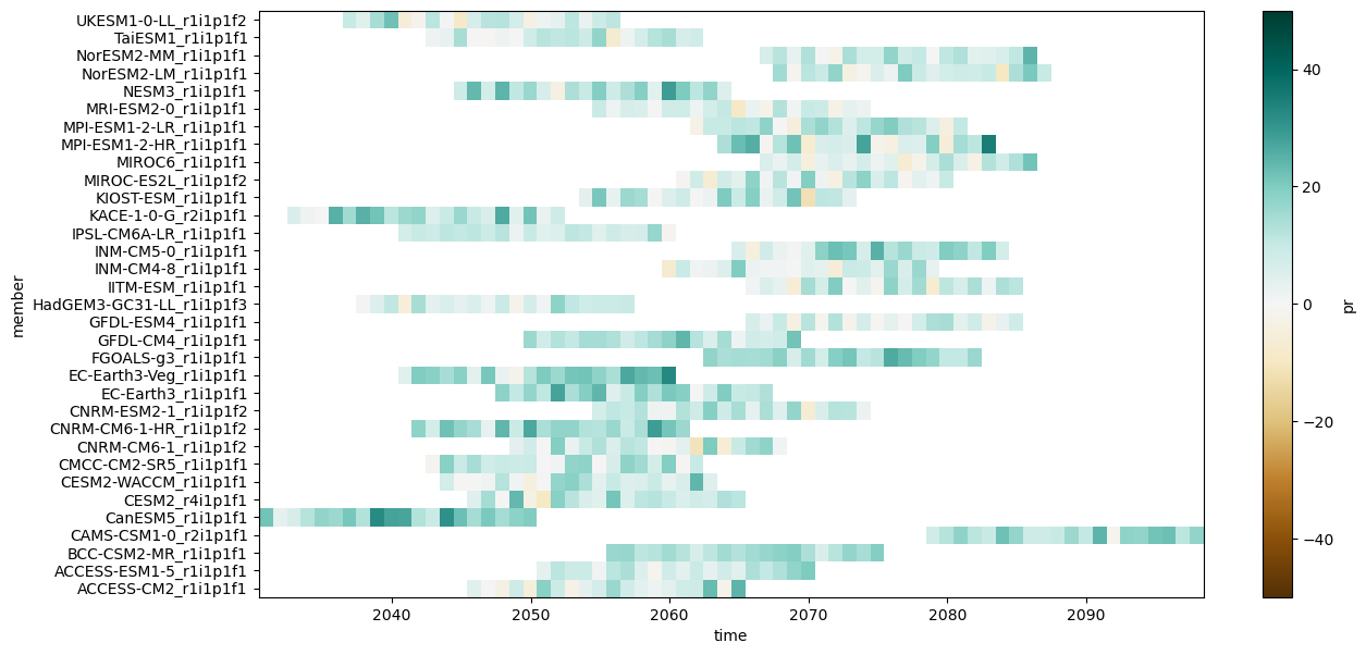
Regional stripes#
Here is an example of generating regional stripes.
cmip6_ssp585_y = cmip6_ssp585["pr"].resample(time="QS-DEC").mean()
cmip6_ssp585_y = cmip6_ssp585_y.sel(time=cmip6_ssp585_y["time"].dt.month==12)

cmip6_hist_c = cmip6_hist["pr"].mean(["time"])

year_delta = cmip6_ssp585_y - cmip6_hist_c
year_delta_rel = year_delta / cmip6_hist_c * 100

regional_mean = year_delta_rel.mean(["lat", "lon"])
regional_mean.plot.imshow(
    figsize=(14,7),
    add_colorbar=True,
    cmap="BrBG",
    vmin=-50,vmax=50)
plt.savefig("regional-stripes-pr.pdf", bbox_inches="tight")
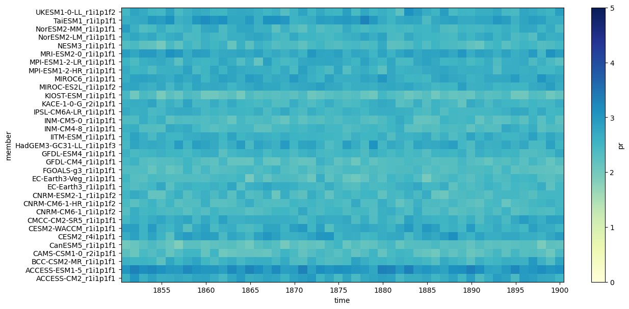
cmip6_hist_y = cmip6_hist["pr"].resample(time="QS-DEC").mean()
cmip6_hist_y = cmip6_hist_y.sel(time=cmip6_hist_y["time"].dt.month==12)

cmip6_hist_y.mean(["lat", "lon"]).plot.imshow(
    figsize=(14,7),
    add_colorbar=True,
    cmap="YlGnBu",
    vmin=0,vmax=5)
<matplotlib.image.AxesImage at 0x7adaaa10cfd0>
We may omit the color bar to display only the spawn of each model time series.
regional_mean.where(np.isnan(regional_mean), 0).plot.imshow(
    figsize=(14,7),
    add_colorbar=False)
<matplotlib.image.AxesImage at 0x7adaaa141b90>