Getting started#
This notebook is a reproducibility example of the IPCC-WGI AR6 Interactive Atlas products. This work is licensed under a Creative Commons Attribution 4.0 International License.

E. Cimadevilla (Santander Meteorology Group. Institute of Physics of Cantabria, CSIC-UC, Spain).
This guideline is structured to assist you in harnessing the wealth of resources available within the IPCC AR6 Interactive Atlas Datalab, enabling you to conduct meaningful climate research and analysis. The datalab serves as a reproducibility platform for the IPCC-WG-AR6 Interactive Atlas products, facilitating not only the reproducibility but also the reusability of the underlying data. It offers transparent access to a wide range of climate-related materials and data, thereby promoting robust scientific investigations and supporting climate change assessment efforts.
Contents in this notebook#
Aim and motivation
Description of the available material within the IPCC-Hub
Data loading and basic data operations
3.1. Initial Data Exploration Plots
3.2. Calculation of anomalies (future projections - historical simulations)
3.3. Spatial aggregation
import os
import xarray
import numpy as np
import pandas as pd
import cartopy.crs as ccrs
import matplotlib.pyplot as plt
1. Aim and motivation#
The IPCC AR6 Interactive Atlas Datalab aims to support the reproducibility and reusability of the data underlying the Interactive Atlas of the IPCC-WGI.
It leverages the latest technologies to provide an efficient research environment that accelerates data analysis. This is achieved by integrating data storage and computational resources with ready-to-use software frameworks.
By utilizing these new technologies, climate data analysis can become more efficient, and the legacy of project results can be extended for the benefit of society.
2. Description of the available material within the datalab#
The datalab is more than just a computing resource; it encompasses data, software, and notebooks that facilitate the reproducibility of the IPCC-WGI AR6 Atlas results. Additionally, this material enables the reusability of data, thereby extending the analysis provided by the IPCC-WGI Interactive Atlas.
Data#
The inventory (data_inventory.csv) catalogs the list of files of the the IPCC-WGI AR6 Interactive Atlas Dataset, originally published at DIGITAL.CSIC for the long-term archival, and also available through the Copernicus Data Store (CDS).
df = pd.read_csv("../../data_inventory.csv")
df.head()
| location | type | variable | project | experiment | frequency | |
|---|---|---|---|---|---|---|
| 0 | https://hub.climate4r.ifca.es/thredds/dodsC/ip... | opendap | pr | CORDEX-ANT | historical | mon |
| 1 | https://hub.climate4r.ifca.es/thredds/dodsC/ip... | opendap | tn | CORDEX-ANT | historical | mon |
| 2 | https://hub.climate4r.ifca.es/thredds/dodsC/ip... | opendap | rx1day | CORDEX-ANT | historical | mon |
| 3 | https://hub.climate4r.ifca.es/thredds/dodsC/ip... | opendap | tx | CORDEX-ANT | historical | mon |
| 4 | https://hub.climate4r.ifca.es/thredds/dodsC/ip... | opendap | txx | CORDEX-ANT | historical | mon |
To open a file, find the location of your dataset in the inventory and open it with xarray.
subset = df.query('type == "opendap" & variable == "pr" & project == "CMIP6" & experiment == "historical"')
location = subset["location"].iloc[0]
location
'https://hub.climate4r.ifca.es/thredds/dodsC/ipcc/ar6/atlas/ia-monthly/CMIP6/historical/pr_CMIP6_historical_mon_185001-201412.nc'
cmip6_historical_pr = xarray.open_dataset(location)
cmip6_historical_pr["pr"]
<xarray.DataArray 'pr' (member: 34, time: 1980, lat: 180, lon: 360)>
[4362336000 values with dtype=float32]
Coordinates:
  * member   (member) |S64 b'CSIRO-ARCCSS_ACCESS-CM2_r1i1p1f1' ... b'MOHC_UKE...
  * time     (time) datetime64[ns] 1850-01-01 1850-02-01 ... 2014-12-01
  * lat      (lat) float64 -89.5 -88.5 -87.5 -86.5 -85.5 ... 86.5 87.5 88.5 89.5
  * lon      (lon) float64 -179.5 -178.5 -177.5 -176.5 ... 177.5 178.5 179.5
Attributes:
    standard_name:  lwe_thickness_of_precipitation_amount
    units:          mm
    cell_methods:   time: sum within days time: mean over days area: mean
    long_name:      Monthly mean of daily accumulated precipitation
    comment:        Monthly mean of daily accumulated precipitation of liquid...
    grid_mapping:   crs
_ChunkSizes: [ 1 1 180 360]Or the description of the index, the corresponding units and the time resolution.
cmip6_historical_pr["pr"].attrs
{'standard_name': 'lwe_thickness_of_precipitation_amount',
 'units': 'mm',
 'cell_methods': 'time: sum within days time: mean over days area: mean',
 'long_name': 'Monthly mean of daily accumulated precipitation',
 'comment': 'Monthly mean of daily accumulated precipitation of liquid water equivalent from all phases',
 'grid_mapping': 'crs',
 '_ChunkSizes': array([  1,   1, 180, 360], dtype=int32)}
Please be aware that some variables pertains to an annual index, whereas the majority of variables and indices are on a monthly basis. For instance, the extreme precipitation:
cmip6_historical_pr["time"][:10]
<xarray.DataArray 'time' (time: 10)>
array(['1850-01-01T00:00:00.000000000', '1850-02-01T00:00:00.000000000',
       '1850-03-01T00:00:00.000000000', '1850-04-01T00:00:00.000000000',
       '1850-05-01T00:00:00.000000000', '1850-06-01T00:00:00.000000000',
       '1850-07-01T00:00:00.000000000', '1850-08-01T00:00:00.000000000',
       '1850-09-01T00:00:00.000000000', '1850-10-01T00:00:00.000000000'],
      dtype='datetime64[ns]')
Coordinates:
  * time     (time) datetime64[ns] 1850-01-01 1850-02-01 ... 1850-10-01
Attributes:
    standard_name:  time
    axis:           T
    long_name:      time
    bounds:         time_bnds
_ChunkSizes: 19803. Data loading and basic data operations#
xarray supports direct serialization and IO to several file formats, from simple Pickle files to the more flexible netCDF format (recommended). Refer to the documentation for further details.
cmip6_hist = xarray.open_dataset(location).sel(
    lon=slice(-10,4),
    lat=slice(36,44),
    time=slice("18500101", "19001231"))

# Summer
cmip6_hist = cmip6_hist.sel(time=(cmip6_hist.time.dt.month.isin([6,7,8])))
cmip6_hist["pr"]
<xarray.DataArray 'pr' (member: 34, time: 153, lat: 8, lon: 14)>
[582624 values with dtype=float32]
Coordinates:
  * member   (member) |S64 b'CSIRO-ARCCSS_ACCESS-CM2_r1i1p1f1' ... b'MOHC_UKE...
  * time     (time) datetime64[ns] 1850-06-01 1850-07-01 ... 1900-08-01
  * lat      (lat) float64 36.5 37.5 38.5 39.5 40.5 41.5 42.5 43.5
  * lon      (lon) float64 -9.5 -8.5 -7.5 -6.5 -5.5 ... -0.5 0.5 1.5 2.5 3.5
Attributes:
    standard_name:  lwe_thickness_of_precipitation_amount
    units:          mm
    cell_methods:   time: sum within days time: mean over days area: mean
    long_name:      Monthly mean of daily accumulated precipitation
    comment:        Monthly mean of daily accumulated precipitation of liquid...
    grid_mapping:   crs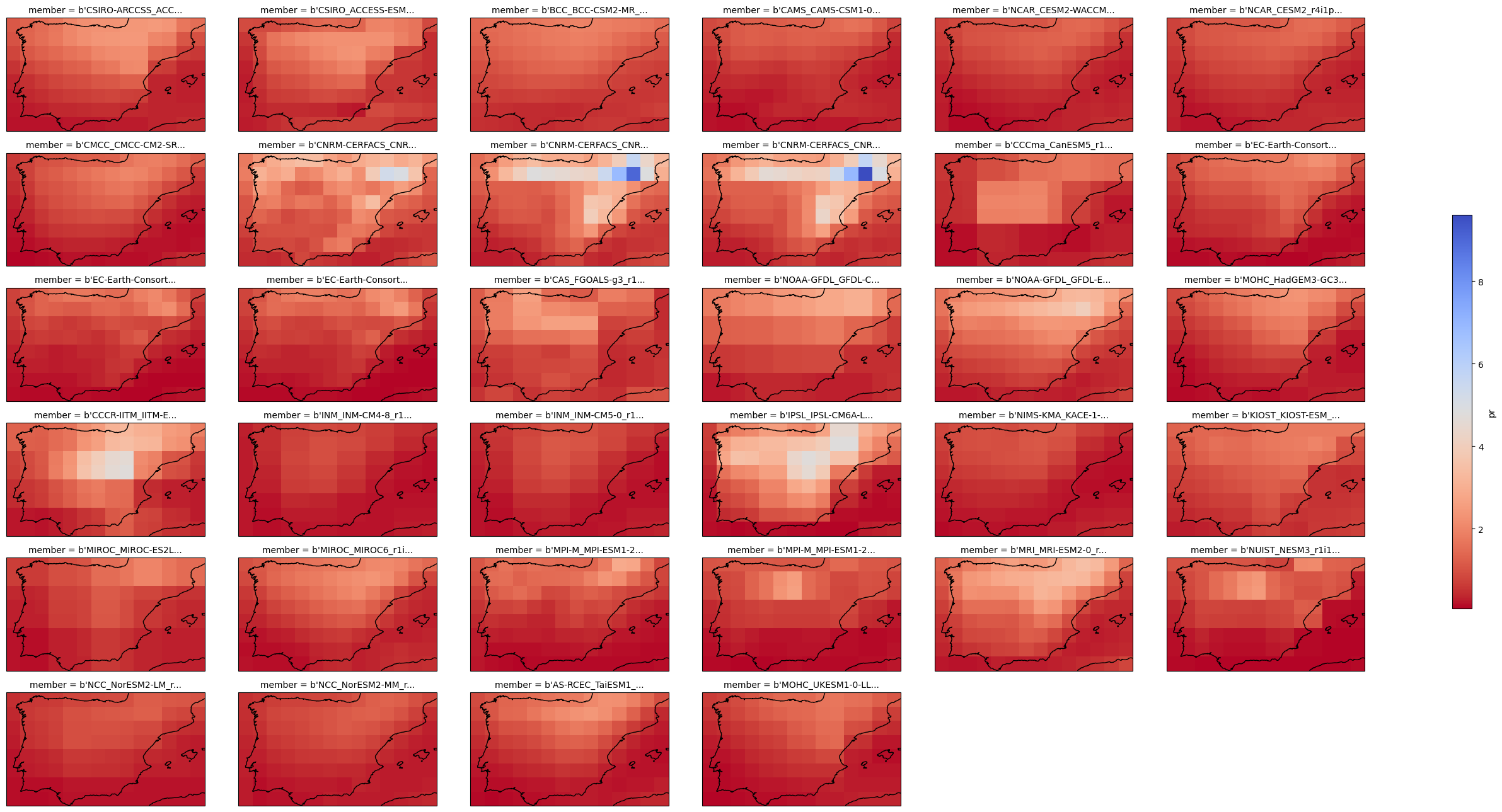
_ChunkSizes: [ 1 1 180 360]3.1. Initial Data Exploration Plots#
xarray allow to easily compute statistics accross the dimensions of the data arrays and plotting the results. Refer to the documentation for further details on computing and plotting.
plot = cmip6_hist["pr"].mean("time").plot(
    x="lon", y="lat", col="member", col_wrap=6,
    figsize=(28,13),
    add_colorbar=True,
    cmap="coolwarm_r",
    cbar_kwargs={"shrink": .5},
    subplot_kws=dict(projection=ccrs.PlateCarree(central_longitude=0)),
    transform=ccrs.PlateCarree())

for ax in plot.axs.flatten():
    ax.coastlines()
    ax.set_extent((-10,4,36,44), ccrs.PlateCarree())
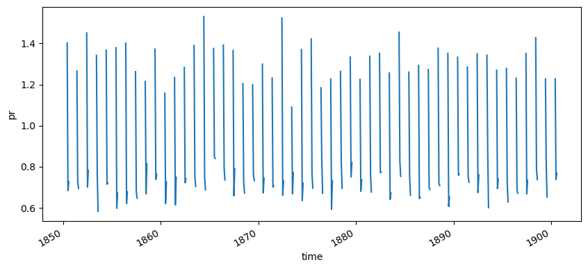
We could also display the temporal series for the original monthly values…
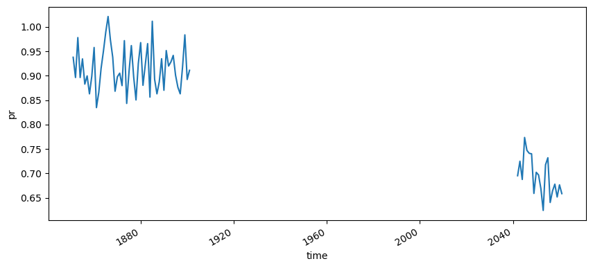
cmip6_hist["pr"].mean(["lat", "lon", "member"]).reindex(time=cmip6_historical_pr["time"]).plot(figsize=(10,4))
[<matplotlib.lines.Line2D at 0x7a15e8539590>]
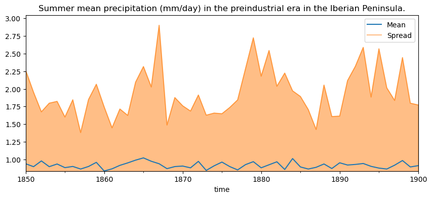
…or the aggregated yearly values.
avg = cmip6_hist["pr"].resample({"time": "Y"}).mean().mean(["lat", "lon", "member"])
spread = (
    cmip6_hist["pr"].mean(["lat", "lon"]).resample({"time": "Y"}).mean().max(["member"]) -
    cmip6_hist["pr"].mean(["lat", "lon"]).resample({"time": "Y"}).mean().min(["member"]))

stats = xarray.concat([avg,spread], "stat").assign_coords({"stat": ["avg", "spread"]}).to_dataframe().reset_index()
fig, ax = plt.subplots(1,1, figsize=(10, 4))

stats[stats["stat"]=="avg"].plot.line(x="time", y="pr", ax=ax)
stats[stats["stat"]=="spread"].plot.area(x="time", y="pr", ax=ax, alpha = .5)

plt.ylim(bottom=stats["pr"].min())
plt.legend(["Mean", "Spread"])
plt.title("Summer mean precipitation (mm/day) in the preindustrial era in the Iberian Peninsula.")
Text(0.5, 1.0, 'Summer mean precipitation (mm/day) in the preindustrial era in the Iberian Peninsula.')
3.2. Calculation of anomalies (future projections - historical simulations)#
We will now calculate the relative precipitation anomaly of a fixed future period (e.g. 2041-2060) relative to the preindustrial period. We will consider the SSP585 mitigation scenario.
subset = df.query('type == "opendap" & variable == "pr" & project == "CMIP6" & experiment == "ssp585"')
location = subset["location"].iloc[0]

cmip6_fut = xarray.open_dataset(location).sel(
    lon=slice(-10,4),
    lat=slice(36,44),
    time=slice("20410101", "20601231"))

# Summer
cmip6_fut = cmip6_fut.sel(time=(cmip6_fut.time.dt.month.isin([6,7,8])))
cmip6_fut["pr"]
<xarray.DataArray 'pr' (member: 33, time: 60, lat: 8, lon: 14)>
[221760 values with dtype=float32]
Coordinates:
  * member   (member) |S64 b'CSIRO-ARCCSS_ACCESS-CM2_r1i1p1f1' ... b'MOHC_UKE...
  * time     (time) datetime64[ns] 2041-06-01 2041-07-01 ... 2060-08-01
  * lat      (lat) float64 36.5 37.5 38.5 39.5 40.5 41.5 42.5 43.5
  * lon      (lon) float64 -9.5 -8.5 -7.5 -6.5 -5.5 ... -0.5 0.5 1.5 2.5 3.5
Attributes:
    standard_name:  lwe_thickness_of_precipitation_amount
    units:          mm
    cell_methods:   time: sum within days time: mean over days area: mean
    long_name:      Monthly mean of daily accumulated precipitation
    comment:        Monthly mean of daily accumulated precipitation of liquid...
    grid_mapping:   crs
_ChunkSizes: [ 1 1 180 360]We can combine the output with the historical data in the same time-series plot:
cmip6_hist.combine_first(cmip6_fut)["pr"].resample({"time": "Y"}).mean().mean(["member", "lat", "lon"]).plot(figsize=(10,4))
[<matplotlib.lines.Line2D at 0x7a15e85b48d0>]
Now we can calculate the anomaly by computing the difference between both climatologies:
anom = cmip6_fut["pr"].mean("time") - cmip6_hist["pr"].mean("time")
rel_anom = anom / cmip6_hist.mean("time") * 100
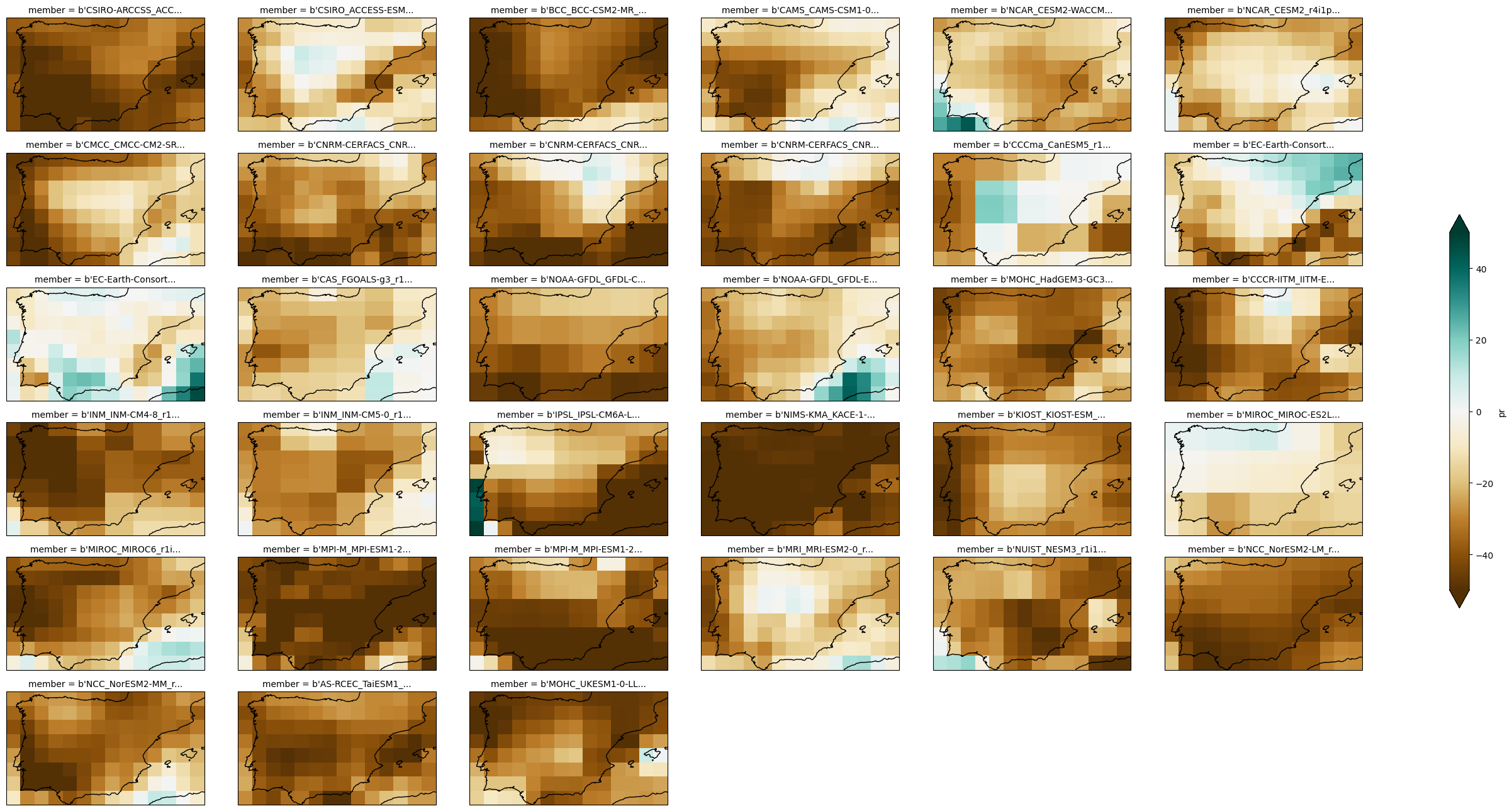
Finally, we can plot the output using an appropriate palette:
plot = rel_anom["pr"].plot(
    x="lon", y="lat", col="member", col_wrap=6,
    figsize=(28,13),
    add_colorbar=True,
    cmap="BrBG",
    cbar_kwargs={"shrink": .5},
    vmin=-50, vmax=50,
    subplot_kws=dict(projection=ccrs.PlateCarree(central_longitude=0)),
    transform=ccrs.PlateCarree())

for ax in plot.axs.flatten():
    ax.coastlines()
    ax.set_extent((-10,4,36,44), ccrs.PlateCarree())
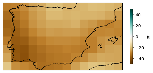
We can do the same for the multi-model ensemble mean.
plot = rel_anom["pr"].mean("member").plot(
    add_colorbar=True,
    cmap="BrBG",
    cbar_kwargs={"shrink": .5},
    vmin=-50, vmax=50,
    subplot_kws=dict(projection=ccrs.PlateCarree(central_longitude=0)),
    transform=ccrs.PlateCarree())

plot.axes.coastlines()
<cartopy.mpl.feature_artist.FeatureArtist at 0x7a15e8a42210>
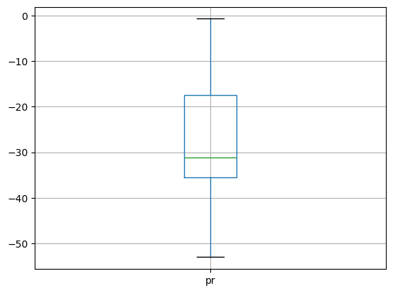
3.3. Spatial aggregation#
The time series plots we have created above, automatically performs spatial aggregations. However, we can calculate weighted values according to the latitude.
weights =  np.cos(np.deg2rad(rel_anom["lat"]))
rel_anom_regional_mean = rel_anom.weighted(weights).mean(["lat", "lon"])
print("Mean: %2.2f\nP25: %2.2f\nP75: %2.2f" % (
    rel_anom_regional_mean["pr"].mean().item(),
    rel_anom_regional_mean["pr"].quantile(.25).item(),
    rel_anom_regional_mean["pr"].quantile(.75).item()))
Mean: -27.98
P25: -35.44
P75: -17.38
rel_anom_regional_mean["pr"].to_dataframe().boxplot()
<Axes: >