Regional averaging of climate information#
This notebook is a reproducibility example of the IPCC-WGI AR6 Interactive Atlas products. This work is licensed under a Creative Commons Attribution 4.0 International License.

M. Iturbide (Santander Meteorology Group. Instituto de Física de Cantabria, CSIC-UC, Santander, Spain).
This notebook is a reproducibility example for the IPCC-WGI AR6 Interactive Atlas products.
This notebook works with the data available in this Hub. In particular, the IPCC-WGI AR6 Interactive Atlas Dataset, originally published at DIGITAL.CSIC for the long-term archival, and also available through the Copernicus Data Store (CDS).
Open the Getting_started.ipynb for a description of the available data and for a quick **introduction to the climate4R framework, the bundle of R packages used in this notebook.
Contents in this notebook#
Libraries
Data preparation
Application of a land-sea mask
Generate regionalized information
Before we start, or at any stage of the notebook, we can customize the plotting area within this notebook as follows:
library(repr)
# Change plot size
options(repr.plot.width=16, repr.plot.height=6)
1. Libraries#
library(loadeR)
library(transformeR)
library(visualizeR)
library(geoprocessoR)
library(rgdal)
library(lattice)
library(magrittr)
library(RColorBrewer)
library(curl)
Loading required package: rJava

Loading required package: loadeR.java

Java version 20x amd64 by N/A detected

NetCDF Java Library v4.6.0-SNAPSHOT (23 Apr 2015) loaded and ready

Loading required package: climate4R.UDG

climate4R.UDG version 0.2.6 (2023-06-26) is loaded

Please use 'citation("climate4R.UDG")' to cite this package.

loadeR version 1.8.2 (2024-06-04) is loaded

Please use 'citation("loadeR")' to cite this package.
    _______   ____  ___________________  __  ________
   / ___/ /  / /  |/  / __  /_  __/ __/ / / / / __  /
  / /  / /  / / /|_/ / /_/ / / / / __/ / /_/ / /_/_/
 / /__/ /__/ / /  / / __  / / / / /__ /___  / / \ \
 \___/____/_/_/  /_/_/ /_/ /_/  \___/    /_/\/   \_\

      github.com/SantanderMetGroup/climate4R
transformeR version 2.2.2 (2023-10-26) is loaded

WARNING: Your current version of transformeR (v2.2.2) is not up-to-date

Get the latest stable version (2.2.3) using <devtools::install_github('SantanderMetGroup/transformeR')>

Please see 'citation("transformeR")' to cite this package.

visualizeR version 1.6.4 (2023-10-26) is loaded

Please see 'citation("visualizeR")' to cite this package.

Please note that rgdal will be retired during October 2023,
plan transition to sf/stars/terra functions using GDAL and PROJ
at your earliest convenience.
See https://r-spatial.org/r/2023/05/15/evolution4.html and https://github.com/r-spatial/evolution
rgdal: version: 1.6-7, (SVN revision 1203)
Geospatial Data Abstraction Library extensions to R successfully loaded
Loaded GDAL runtime: GDAL 3.8.0, released 2023/11/06
Path to GDAL shared files:
 GDAL does not use iconv for recoding strings.
GDAL binary built with GEOS: TRUE
Loaded PROJ runtime: Rel. 9.3.0, September 1st, 2023, [PJ_VERSION: 930]
Path to PROJ shared files: /home/zequi/.local/share/proj:/home/zequi/miniconda3/share/proj
PROJ CDN enabled: TRUE
Linking to sp version:2.1-1
To mute warnings of possible GDAL/OSR exportToProj4() degradation,
use options("rgdal_show_exportToProj4_warnings"="none") before loading sp or rgdal.

geoprocessoR version 0.2.2 (2023-06-22) is loaded

Please see 'citation("geoprocessoR")' to cite this package.

Loading required package: sp
2. Data Preparation#
The aim of this notebook is to illustrate the operations that can be carried out in climate4R to synthesize climate information through regionalized statistics. These operations can be applied to any climate4R (C4R) grid, containing any type of information. Here, we will demonstrate this using a simple data loading operation to obtain the target C4R grid. For more detailed explanations on data loading, please refer to other notebooks (e.g., getting started).
data.paths <- read.csv("../../../data_inventory.csv")
str(data.paths)
'data.frame':	1726 obs. of  6 variables:
 $ location  : chr  "https://hub.climate4r.ifca.es/thredds/dodsC/ipcc/ar6/atlas/ia-monthly/CORDEX-ANT/historical/pr_CORDEX-ANT_histo"| __truncated__ "https://hub.climate4r.ifca.es/thredds/dodsC/ipcc/ar6/atlas/ia-monthly/CORDEX-ANT/historical/tn_CORDEX-ANT_histo"| __truncated__ "https://hub.climate4r.ifca.es/thredds/dodsC/ipcc/ar6/atlas/ia-monthly/CORDEX-ANT/historical/rx1day_CORDEX-ANT_h"| __truncated__ "https://hub.climate4r.ifca.es/thredds/dodsC/ipcc/ar6/atlas/ia-monthly/CORDEX-ANT/historical/tx_CORDEX-ANT_histo"| __truncated__ ...
 $ type      : chr  "opendap" "opendap" "opendap" "opendap" ...
 $ variable  : chr  "pr" "tn" "rx1day" "tx" ...
 $ project   : chr  "CORDEX-ANT" "CORDEX-ANT" "CORDEX-ANT" "CORDEX-ANT" ...
 $ experiment: chr  "historical" "historical" "historical" "historical" ...
 $ frequency : chr  "mon" "mon" "mon" "mon" ...
locationrefers to the pathtyperefers to the access mode, local (netcdf) or remote (opendap).variablereferst to the climatic variable or index (i.e. tas, pr, tn, rx1day, etc.)projectrefers to the project coordinating the datasets (i.e. CORDEX-EUR, CMIP5, CMIP6, etc.)experimentreferst to the scenario (i.e. historical, rcp26, ssp126, rcp85, etc.)
We can easily apply filters to narrow down to the desired file. In this example the TXx index (maximum of maximum temperatures) from CMIP6, for the historical and ssp370 experiments. The information piece we need is the location.
nc.file.ssp370 <- subset(data.paths, project == "CMIP6" & type == "netcdf" & variable == "txx" & experiment == "ssp370")[["location"]]
nc.file.hist <- subset(data.paths, project == "CMIP6" & type == "netcdf" & variable == "txx" & experiment == "historical")[["location"]]
Before loading the data, we can set common parameters such as the geographical domain, the target season (boreal summer in this example), the reference period for the historical baseline (in this case, the pre-industrial period) and the future period (in this case, the medioum term).
ref.period <- 1850:1900
fut.period <- 2041:2060
lonLim <- c(-11, 40)
latLim <- c(25, 50)
season <- 6:8
Now we load the data for the historical and ssp585 experiments.
cmip6.hist <- loadGridData(nc.file.hist,
                         var = "txx",
                         lonLim = lonLim,
                         latLim = latLim,
                         years = ref.period,
                         season = season)  %>% suppressWarnings
[2024-11-07 10:36:51.249873] Defining geo-location parameters

[2024-11-07 10:36:51.795392] Defining time selection parameters

[2024-11-07 10:36:51.84402] Retrieving data subset ...

[2024-11-07 10:37:05.282443] Done
cmip6.ssp370 <- loadGridData(nc.file.ssp370,
                         var = "txx",
                         lonLim = lonLim,
                         latLim = latLim,
                         years = fut.period,
                         season = season)  %>% suppressWarnings
[2024-11-07 10:37:05.451922] Defining geo-location parameters

[2024-11-07 10:37:05.51715] Defining time selection parameters

[2024-11-07 10:37:05.541033] Retrieving data subset ...

[2024-11-07 10:37:09.102625] Done
Before continuing, we must retain the same models (in the same order) in both the future and historical grids. To do so, we apply the intersectGrid function.
cmip6.common.mems <- intersectGrid(cmip6.hist, cmip6.ssp370, type = "members", which.return = 1:2)
cmip6.hist <- cmip6.common.mems[[1]] ; cmip6.ssp370 <- cmip6.common.mems[[2]]
It is always a good practice to make sure that the members in both grids are identical:
identical(cmip6.hist$Members, cmip6.ssp370$Members)
Calculate the climate change signal with the gridArithmetics function.
delta <- gridArithmetics(climatology(cmip6.ssp370), climatology(cmip6.hist), operator = "-")
[2024-11-07 10:37:09.278633] - Computing climatology...

[2024-11-07 10:37:09.528503] - Done.

[2024-11-07 10:37:09.996502] - Computing climatology...

[2024-11-07 10:37:10.319743] - Done.
Plot the map with spatialPlot.
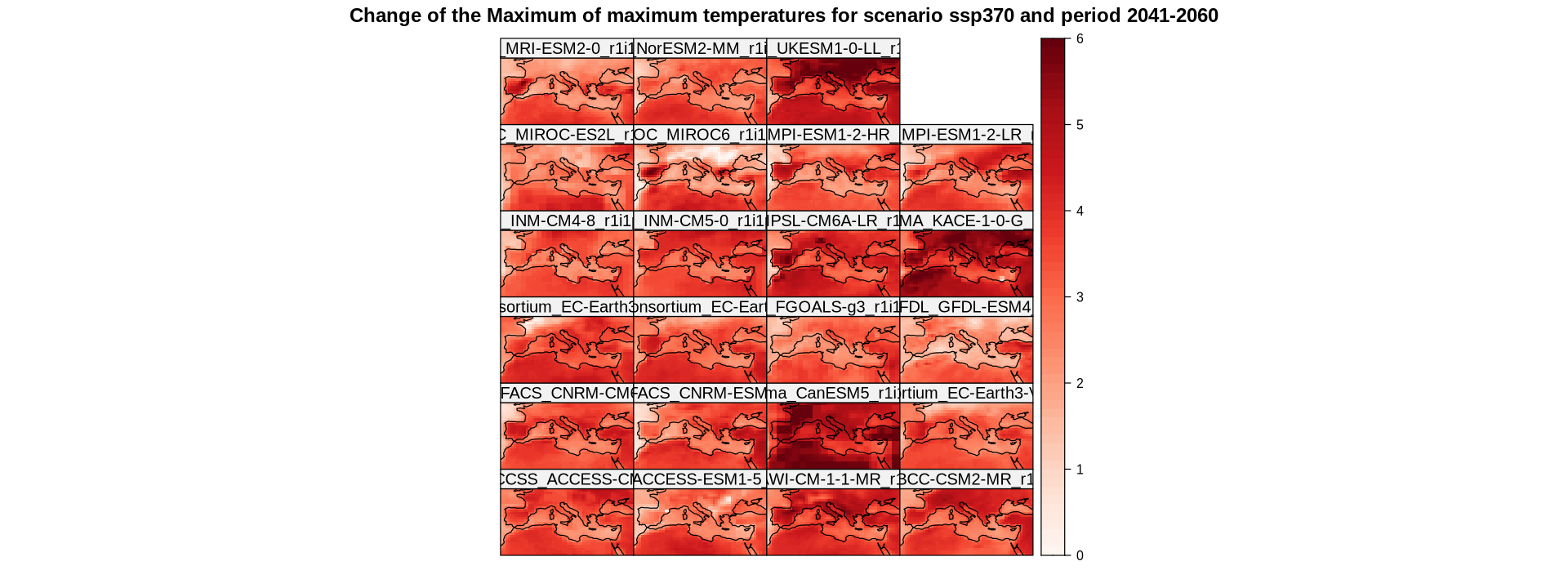
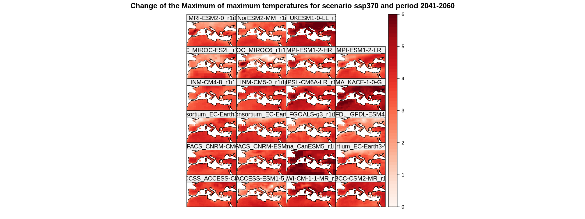
spatialPlot(delta,
            backdrop.theme = "coastline",
            at = seq(0, 6, 0.1),
            set.max = 6,
            set.min = 0,
            color.theme = "Reds",
            main = "Change of the Maximum of maximum temperatures for scenario ssp370 and period 2041-2060",
            strip = strip.custom(factor.levels = delta$Members))
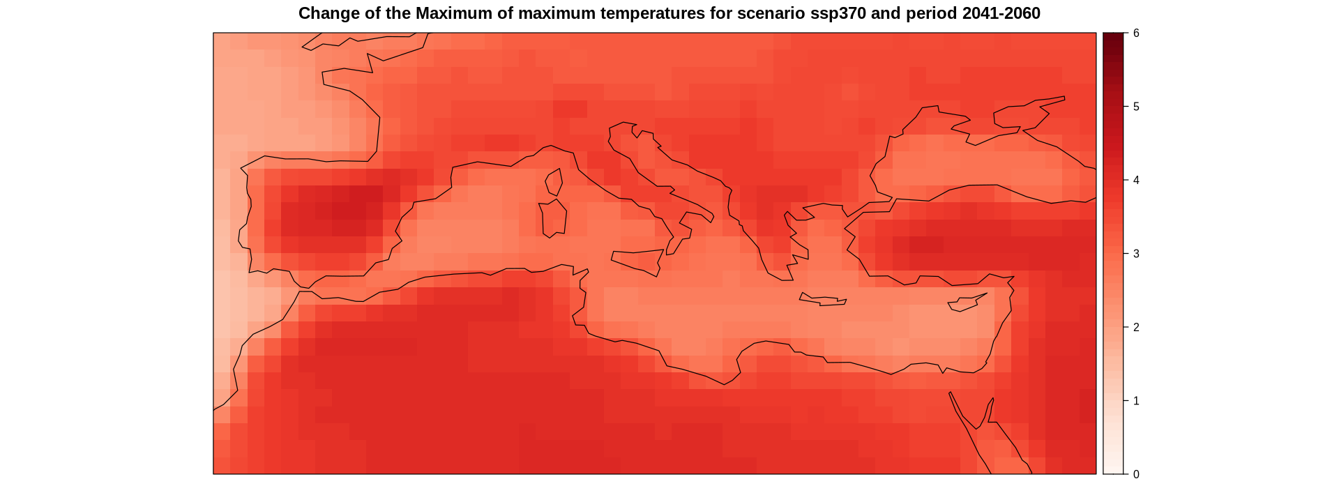
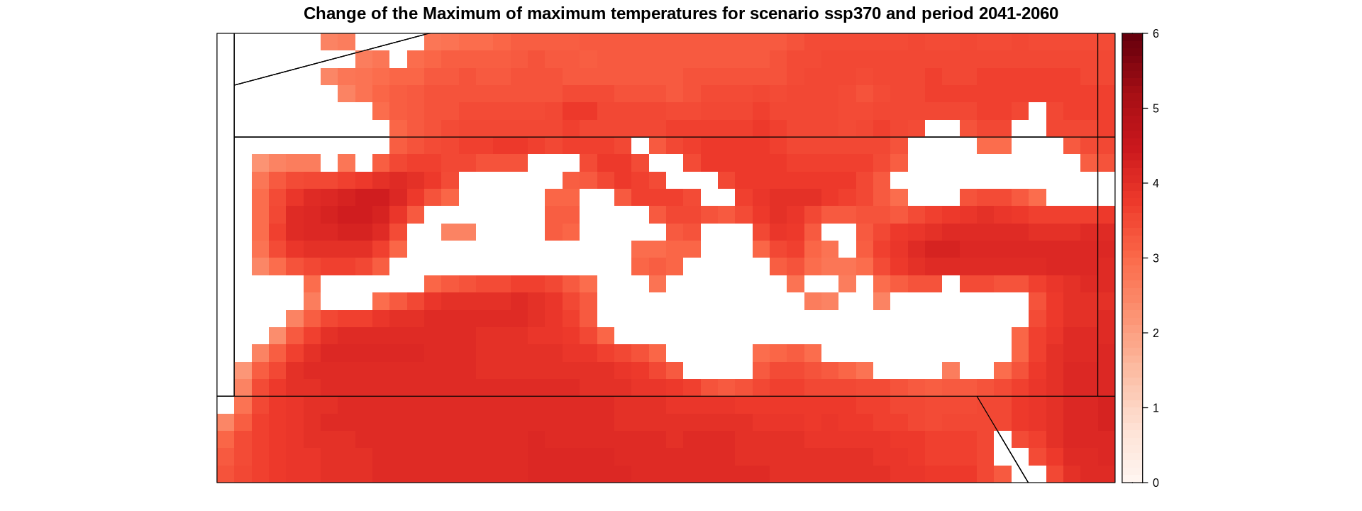
Calculate and plot the map of the ensemble mean.
delta.ens.mean <- aggregateGrid(delta, aggr.mem = list(FUN = mean))
[2024-11-07 10:37:14.472943] - Aggregating members...

[2024-11-07 10:37:14.48203] - Done.
spatialPlot(delta.ens.mean,
            backdrop.theme = "coastline",
            at = seq(0, 6, 0.1),
            set.max = 6,
            set.min = 0,
            color.theme = "Reds",
            main = "Change of the Maximum of maximum temperatures for scenario ssp370 and period 2041-2060",
            strip = strip.custom(factor.levels = delta$Members))
3. Application of a land-sea mask#
The land-sea masks necessary for this dataset are accessible in the IPCC-WGI/Atlas GitHub repository, which is mirrored here. Given that the CMIP6 data within the IPCC-WGI AR6 Interactive Atlas dataset adopts a consistent 1-degree grid, it is essential to reference the 1-degree mask (land_sea_mask_1degree.nc4) located in the same GitHub repository where the warming level information is available, this is the IPCC-WGI/Atlas GitHub repository. Therefore we can load this mask also remotely and using the lonLim and latLim parameters defined previously.
The variable name is sftlf in this case.
url <- "https://github.com/SantanderMetGroup/ATLAS/raw/refs/heads/main/reference-grids/land_sea_mask_1degree.nc4"
temp.file <- tempfile(fileext = ".nc")
curl_download(url, temp.file)
mask <- loadGridData(temp.file,
                    var = "sftlf",
                    lonLim = lonLim,
                    latLim = latLim)
[2024-11-07 14:46:36.966025] Defining geo-location parameters

[2024-11-07 14:46:37.035901] Defining time selection parameters

NOTE: Undefined Dataset Time Axis (static variable)

[2024-11-07 14:46:37.047954] Retrieving data subset ...

[2024-11-07 14:46:37.114017] Done
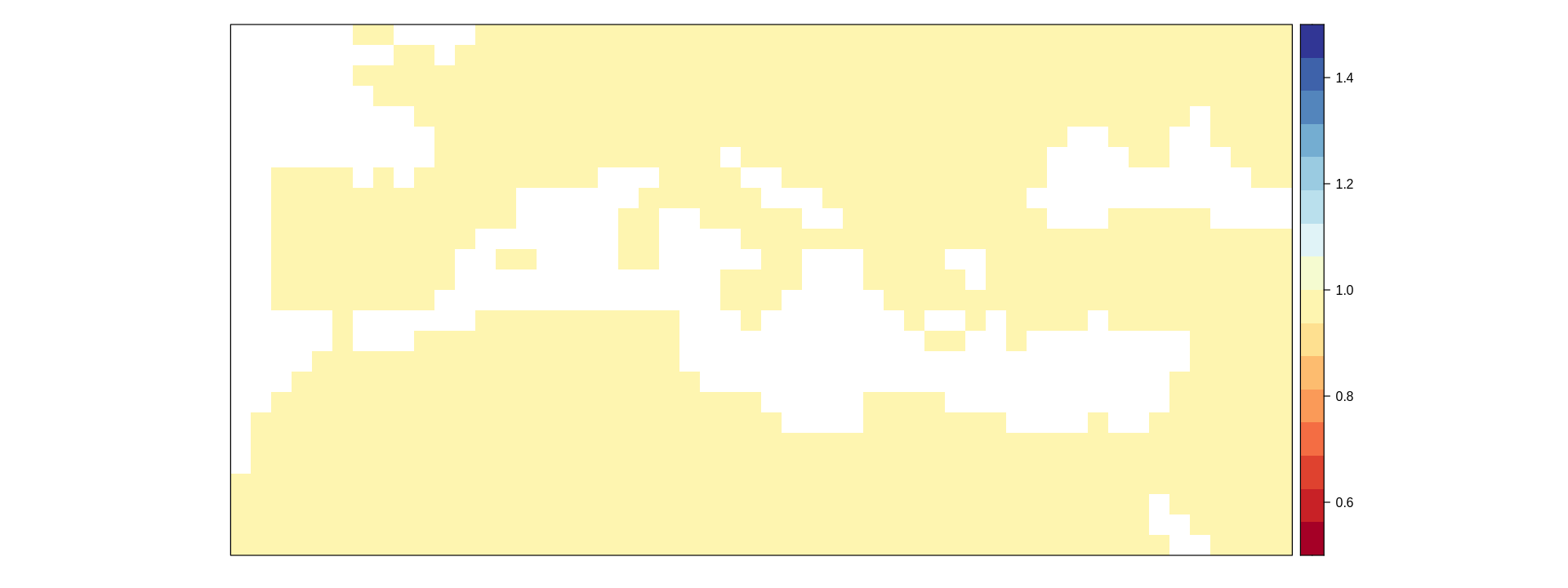
After loading the mask, we need to apply a threshold to the resulting grid to make it binary. In this example, we want to retain the data over the land areas. Therefore, we will set sea grid cells as NA (values below the threshold are positioned first in the values parameter), and land grid cells will be set to 1.
mask <- binaryGrid(mask, condition = "GT", threshold = 0.5, values = c(NA, 1))
spatialPlot(mask)
To apply the mask, we can utilize the gridArithmetics function directly.
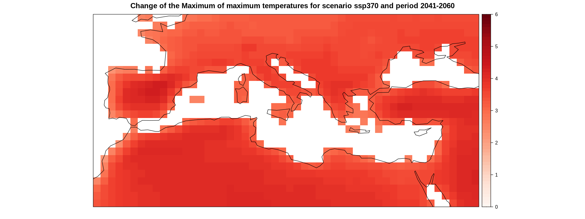
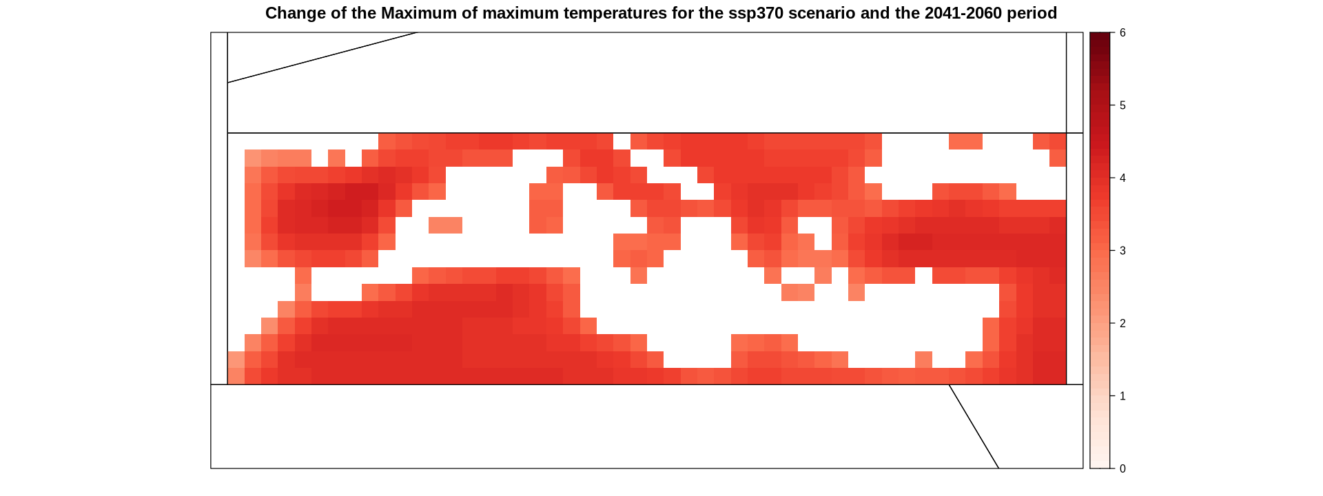
delta.ens.mean.land <- gridArithmetics(delta.ens.mean, mask, operator = "*")
spatialPlot(delta.ens.mean.land,
            backdrop.theme = "coastline",
            at = seq(0, 6, 0.1),
            set.max = 6,
            set.min = 0,
            color.theme = "Reds",
            main = "Change of the Maximum of maximum temperatures for scenario ssp370 and period 2041-2060")
To apply the same mask to the multi-model grid, a trick can be employed to duplicate the mask for each member in the target grid using the rep function. The expression getShape(delta, "member") returns the number of members in the delta grid. The resulting grid is a list with a length equal to the number of members, where each slot contains the same mask grid. Afterwards, binaryGrid is used to bind them all along the member dimension.
multi.mask <- rep(list(mask), getShape(delta, "member")) %>% bindGrid(dimension = "member", skip.temporal.check = T)
Now we are ready to apply gridArithmetics, as the dimension lengths are now the same in both the target grid and the mask grid.
delta.land <- gridArithmetics(delta, multi.mask, operator = "*")
spatialPlot(delta.land,
            backdrop.theme = "coastline",
            at = seq(0, 6, 0.1),
            set.max = 6,
            set.min = 0,
            color.theme = "Reds",
            main = "Change of the Maximum of maximum temperatures for scenario ssp370 and period 2041-2060",
            strip = strip.custom(factor.levels = delta$Members))
4. Generate regionalized information#
To get regionalized outcomes, we could consider any region within our study area. In this example, we use one of the IPCC-WGI Reference Regions available at IPCC-WGI/Atlas GitHub repository.
ref.regs <- readOGR("https://raw.githubusercontent.com/IPCC-WG1/Atlas/refs/heads/main/reference-regions/IPCC-WGI-reference-regions-v4.geojson") %>%
                suppressWarnings
OGR data source with driver: GeoJSON
Source: "https://raw.githubusercontent.com/IPCC-WG1/Atlas/refs/heads/main/reference-regions/IPCC-WGI-reference-regions-v4.geojson", layer: "IPCC-WGI-reference-regions-v4"
with 58 features
It has 5 fields
plot(ref.regs)
text(coordinates(ref.regs)[,1], coordinates(ref.regs)[,2], ref.regs$Acronym)

These regions can be added as a layer when plotting the map with spatialPlot. We do this by passing list(ref.regs, first = FALSE) to the sp.layout parameter. Note that the regions are passed inside a list, where other parameters can be added, such as first = FALSE to overlay the layer on top, or others to adjust line width, color, etc.
spatialPlot(delta.ens.mean.land,
            at = seq(0, 6, 0.1),
            set.max = 6,
            set.min = 0,
            color.theme = "Reds",
            main = "Change of the Maximum of maximum temperatures for scenario ssp370 and period 2041-2060",
            sp.layout = list(ref.regs, first = F))
In this example we are going to focus on the Mediterranean (MED).
med <- subset(ref.regs, Acronym == "MED") %>% as("SpatialPolygons")
The grids here loaded indicate they are “LatLonProjection”:
attr(delta.ens.mean.land$xyCoords, "projection")
The reference regions projections is…
proj4string(med)
Although they may seem different, LatLonProjection in the IA-Dataset is equivalent to +proj=longlat +datum=WGS84 +no_defs. Therefore, we redefine the projection to allow for the subsequent intersection.
attr(delta.ens.mean.land$xyCoords, "projection") <- proj4string(med)
Now we are ready for the intersection. Apply the overGrid function.
delta.ens.mean.land.med <- overGrid(delta.ens.mean.land, layer = med)
spatialPlot(delta.ens.mean.land.med,
            at = seq(0, 6, 0.1),
            set.max = 6,
            set.min = 0,
            color.theme = "Reds",
            main = "Change of the Maximum of maximum temperatures for the ssp370 scenario and the 2041-2060 period",
            sp.layout = list(ref.regs, first = F))
Next, we show an example of generating regional stripes, although other visualizations could also be created. First, we average the data yearly using the aggregateGrid function, which returns yearly data of winter precipitation averages (3-month averages). Next, we calculate the historical climatology to serve as the reference baseline.
Following a similar approach to the one used earlier for the land mask application, we duplicate the historical climatology for each time step in the future yearly data to ensure consistent array dimensions. This allows for calculating yearly anomalies relative to the historical climatology using the gridArithmetics function. In other words, the historical climatology is subtracted from each future year of the projections.
cmip6.ssp370.y <- aggregateGrid(cmip6.ssp370, aggr.y = list(FUN = "mean", na.rm = TRUE))
cmip6.hist.c <- climatology(cmip6.hist)
cmip6.hist.multi.year <- rep(list(cmip6.hist.c), getShape(cmip6.ssp370.y, "time")) %>% bindGrid(dimension = "time")
year.delta <- gridArithmetics(cmip6.ssp370.y, cmip6.hist.multi.year, operator = "-")
[2024-11-07 10:37:24.580067] Performing annual aggregation...

[2024-11-07 10:37:29.598088] Done.

[2024-11-07 10:37:29.659808] - Computing climatology...

[2024-11-07 10:37:30.56635] - Done.
To perform spatial aggregations we only need to apply the function aggregateGrid again but with the appropriate parameters.
regional.mean <- aggregateGrid(year.delta, aggr.spatial = list(FUN = "mean", na.rm = TRUE))
Calculating areal weights...

[2024-11-07 10:37:31.282897] - Aggregating spatially...

[2024-11-07 10:37:31.318585] - Done.
The function stripePlot performs the same spatial aggregation internally and plots the stripes.
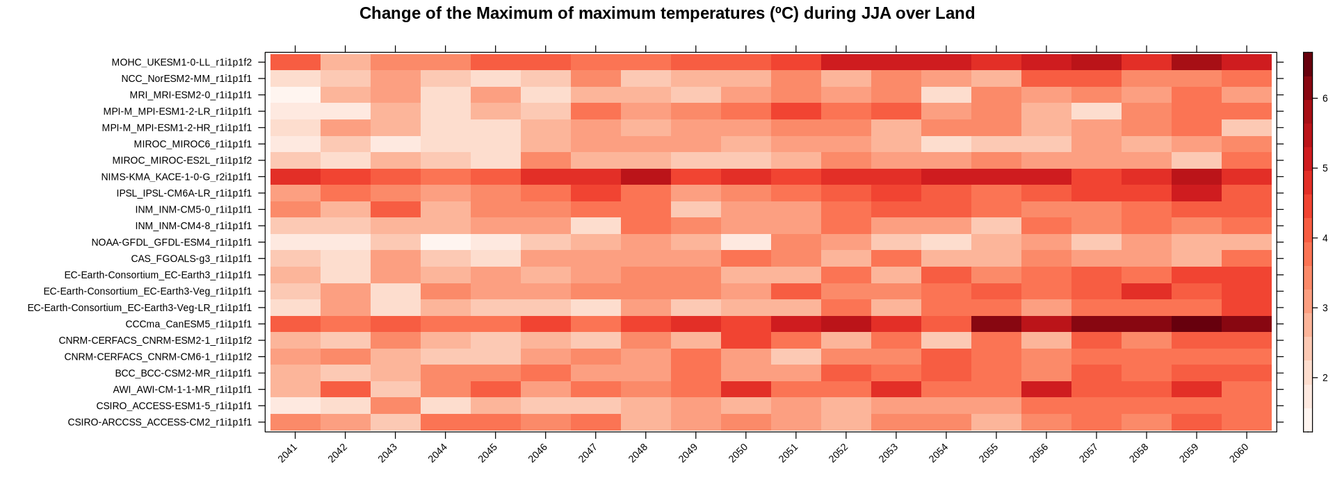
stripePlot(year.delta,
           aggr.spatial = list(FUN = "mean", na.rm = TRUE),
           main = "Change of the Maximum of maximum temperatures (ºC) during JJA over Land",
           color.theme = "Reds",
           rev.colors = FALSE)
Calculating areal weights...

[2024-11-07 10:37:31.344606] - Aggregating spatially...

[2024-11-07 10:37:31.379066] - Done.
Next the stripes of the historical reference are plotted.
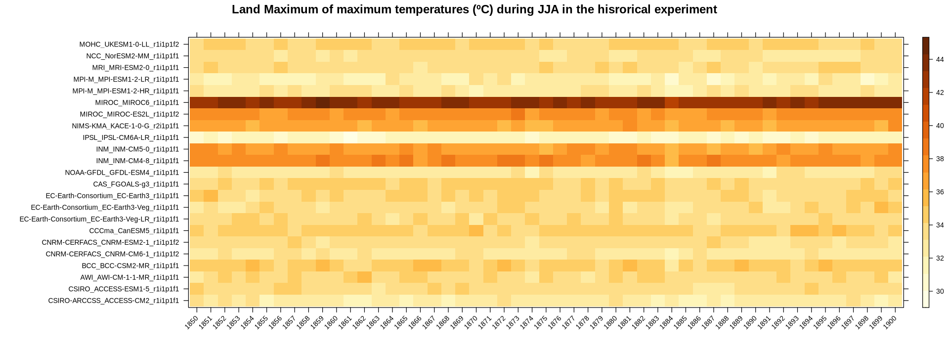
stripePlot(aggregateGrid(cmip6.hist, aggr.y = list(FUN = "mean", na.rm = TRUE)),
           main = "Land Maximum of maximum temperatures (ºC) during JJA in the hisrorical experiment",
           color.theme =  "YlOrBr")
[2024-11-07 10:37:31.582012] Performing annual aggregation...

[2024-11-07 10:37:41.589599] Done.

Calculating areal weights...

[2024-11-07 10:37:41.630434] - Aggregating spatially...

[2024-11-07 10:37:42.266306] - Done.
Session Info#
sessionInfo()
R version 4.3.3 (2024-02-29)
Platform: x86_64-conda-linux-gnu (64-bit)
Running under: Ubuntu 22.04.3 LTS

Matrix products: default
BLAS/LAPACK: /opt/conda/envs/climate4r/lib/libopenblasp-r0.3.27.so;  LAPACK version 3.12.0

locale:
 [1] LC_CTYPE=en_US.UTF-8          LC_NUMERIC=C
 [3] LC_TIME=en_US.UTF-8           LC_COLLATE=en_US.UTF-8
 [5] LC_MONETARY=en_US.UTF-8       LC_MESSAGES=en_US.UTF-8
 [7] LC_PAPER=en_US.UTF-8          LC_NAME=en_US.UTF-8
 [9] LC_ADDRESS=en_US.UTF-8        LC_TELEPHONE=en_US.UTF-8
[11] LC_MEASUREMENT=en_US.UTF-8    LC_IDENTIFICATION=en_US.UTF-8

time zone: Etc/UTC
tzcode source: system (glibc)

attached base packages:
[1] stats     graphics  grDevices utils     datasets  methods   base

other attached packages:
 [1] RColorBrewer_1.1-3  magrittr_2.0.3      lattice_0.22-6
 [4] rgdal_1.6-7         sp_2.1-4            geoprocessoR_0.2.2
 [7] visualizeR_1.6.4    transformeR_2.2.2   loadeR_1.8.1
[10] climate4R.UDG_0.2.6 loadeR.java_1.1.1   rJava_1.0-11
[13] repr_1.1.7

loaded via a namespace (and not attached):
 [1] viridisLite_0.4.2       IRdisplay_1.1           R.utils_2.12.3
 [4] fields_16.2             bitops_1.0-8            fastmap_1.2.0
 [7] RCurl_1.98-1.16         digest_0.6.37           dotCall64_1.1-1
[10] lifecycle_1.0.4         sf_1.0-16               verification_1.42
[13] terra_1.7-78            compiler_4.3.3          CircStats_0.2-6
[16] rlang_1.1.4             tools_4.3.3             utf8_1.2.4
[19] sm_2.2-6.0              data.table_1.15.4       interp_1.1-6
[22] classInt_0.4-10         abind_1.4-5             KernSmooth_2.23-24
[25] pbdZMQ_0.3-13           gdalUtils_2.0.3.2       R.oo_1.26.0
[28] grid_4.3.3              fansi_1.0.6             latticeExtra_0.6-30
[31] SpecsVerification_0.5-3 e1071_1.7-16            colorspace_2.1-1
[34] scales_1.3.0            iterators_1.0.14        MASS_7.3-60.0.1
[37] cli_3.6.3               crayon_1.5.3            DBI_1.2.3
[40] pbapply_1.7-2           proxy_0.4-27            maps_3.4.2
[43] mapplots_1.5.2          parallel_4.3.3          base64enc_0.1-3
[46] vctrs_0.6.5             boot_1.3-31             jsonlite_1.8.9
[49] kohonen_3.0.12          jpeg_0.1-10             foreach_1.5.2
[52] units_0.8-5             glue_1.7.0              spam_2.10-0
[55] dtw_1.23-1              codetools_0.2-20        akima_0.6-3.4
[58] deldir_2.0-4            raster_3.6-26           munsell_0.5.1
[61] pillar_1.9.0            htmltools_0.5.8.1       IRkernel_1.3.2
[64] R6_2.5.1                RcppEigen_0.3.4.0.2     vioplot_0.5.0
[67] evaluate_1.0.0          png_0.1-8               R.methodsS3_1.8.2
[70] class_7.3-22            Rcpp_1.0.13             uuid_1.2-1
[73] easyVerification_0.4.5  padr_0.6.2              zoo_1.8-12