Getting started#
This notebook is a reproducibility example of the IPCC-WGI AR6 Interactive Atlas products. This work is licensed under a Creative Commons Attribution 4.0 International License.

M. Iturbide (Santander Meteorology Group. Institute of Physics of Cantabria, CSIC-UC, Spain).
Welcome to the datalab “Getting Started” notebook! This guideline is structured to assist you in harnessing the wealth of resources available within the IPCC AR6 Interactive Atlas Datalab, enabling you to conduct meaningful climate research and analysis. The datalab serves as a reproducibility platform for the IPCC-WG-AR6 Interactive Atlas products, facilitating not only the reproducibility but also the reusability of the underlying data. It offers transparent access to a wide range of climate-related materials and data, thereby promoting robust scientific investigations and supporting climate change assessment efforts.
This guideline is divided into several sections. We will begin by outlining the overarching aim and motivation behind the datalab, clarifying its purpose and significance in the realm of climate research. Subsequently, we delve into the Description of the available material within the datalab, providing insights into the diverse datasets and resources at your disposal for climate analysis. Finally, in the section on Data loading and basic data operations, we walk you through the fundamental steps required to start working with climate data effectively.
Contents in this notebook#
Aim and motivation
Description of the available material within the datalab
Data loading and basic data operations
3.1. Library loading
3.2. Data loading
3.3. The structure of the climate4R grid
3.4. Initial Data Exploration Plots
3.5. Calculation of anomalies (future projections - historical simulations)
3.6. Spatial aggregation
Before we start, or at any stage of the notebook, we can customize the plotting area within this notebook as follows:
library(repr)
# Change plot size
options(repr.plot.width=18, repr.plot.height=8)
1. Aim and motivation#
The IPCC AR6 Interactive Atlas Datalab aims to support the reproducibility and reusability of the data underlying the Interactive Atlas of the IPCC-WGI. It leverages the latest technologies to provide an efficient research environment that accelerates data analysis. This is achieved by integrating data storage and computational resources with ready-to-use software frameworks. By utilizing these new technologies, climate data analysis can become more efficient, and the legacy of project results can be extended for the benefit of society.
2. Description of the available material within the datalab#
The datalab is more than just a computing resource; it encompasses data (including NcML catalogs), software, and notebooks that facilitate the reproducibility of the IPCC-WGI AR6 Atlas results. Additionally, this material enables the reusability of data, thereby extending the analysis provided by the IPCC-WGI Interactive Atlas.
Software#
The datalab comes with pre-installed ready-to-use software for managing and performing operations with climate data. This software is a collection of R packages known as the climate4R framework (Iturbide et al., 2019. DOI: 10.1016/j.envsoft.2018.09.009), which can be selected from the kernel menu. Go to the climate4R GitHub repository for more information.
For Python users, there is also a python 3 environment available. It’s worth noting, however, that in this case, the pre-installed software is more basic.
The core climate4R libraries that allow for data loading, transformation (e.g. spatio-temporal aggregations), and visualization are loadeR, transformeR and visualizeR.
library(loadeR)
library(transformeR)
library(visualizeR)
Loading required package: rJava

Loading required package: loadeR.java

Java version 20x amd64 by N/A detected

NetCDF Java Library v4.6.0-SNAPSHOT (23 Apr 2015) loaded and ready

Loading required package: climate4R.UDG

climate4R.UDG version 0.2.6 (2023-06-26) is loaded

Please use 'citation("climate4R.UDG")' to cite this package.

loadeR version 1.8.2 (2024-06-04) is loaded

Please use 'citation("loadeR")' to cite this package.
    _______   ____  ___________________  __  ________
   / ___/ /  / /  |/  / __  /_  __/ __/ / / / / __  /
  / /  / /  / / /|_/ / /_/ / / / / __/ / /_/ / /_/_/
 / /__/ /__/ / /  / / __  / / / / /__ /___  / / \ \
 \___/____/_/_/  /_/_/ /_/ /_/  \___/    /_/\/   \_\

      github.com/SantanderMetGroup/climate4R
transformeR version 2.2.2 (2023-10-26) is loaded

WARNING: Your current version of transformeR (v2.2.2) is not up-to-date

Get the latest stable version (2.2.3) using <devtools::install_github('SantanderMetGroup/transformeR')>

Please see 'citation("transformeR")' to cite this package.

visualizeR version 1.6.4 (2023-10-26) is loaded

Please see 'citation("visualizeR")' to cite this package.
However, the software includes the entire climate4R framework and other useful libraries. For instance, it includes the powerful plotting library lattice or the magrittr library for piping operations (through %>%).
library(lattice)
library(magrittr)
Data#
The inventory (data_inventory.csv) catalogs the list of files of the the IPCC-WGI AR6 Interactive Atlas Dataset, originally published at DIGITAL.CSIC for the long-term archival, and also available through the Copernicus Data Store (CDS).
We simply need to read this file with the read.csv function to get the data.frame of this information, which contains four columns: location, type, variable, project, experiment, frequency.
df <- read.csv("../../data_inventory.csv")
head(df)
| location | type | variable | project | experiment | frequency | |
|---|---|---|---|---|---|---|
| <chr> | <chr> | <chr> | <chr> | <chr> | <chr> | |
| 1 | https://hub.climate4r.ifca.es/thredds/dodsC/ipcc/ar6/atlas/ia-monthly/CORDEX-ANT/historical/pr_CORDEX-ANT_historical_mon_197001-200512.nc | opendap | pr | CORDEX-ANT | historical | mon |
| 2 | https://hub.climate4r.ifca.es/thredds/dodsC/ipcc/ar6/atlas/ia-monthly/CORDEX-ANT/historical/tn_CORDEX-ANT_historical_mon_197001-200512.nc | opendap | tn | CORDEX-ANT | historical | mon |
| 3 | https://hub.climate4r.ifca.es/thredds/dodsC/ipcc/ar6/atlas/ia-monthly/CORDEX-ANT/historical/rx1day_CORDEX-ANT_historical_mon_197001-200512.nc | opendap | rx1day | CORDEX-ANT | historical | mon |
| 4 | https://hub.climate4r.ifca.es/thredds/dodsC/ipcc/ar6/atlas/ia-monthly/CORDEX-ANT/historical/tx_CORDEX-ANT_historical_mon_197001-200512.nc | opendap | tx | CORDEX-ANT | historical | mon |
| 5 | https://hub.climate4r.ifca.es/thredds/dodsC/ipcc/ar6/atlas/ia-monthly/CORDEX-ANT/historical/txx_CORDEX-ANT_historical_mon_197001-200512.nc | opendap | txx | CORDEX-ANT | historical | mon |
| 6 | https://hub.climate4r.ifca.es/thredds/dodsC/ipcc/ar6/atlas/ia-monthly/CORDEX-ANT/historical/tnn_CORDEX-ANT_historical_mon_197001-200512.nc | opendap | tnn | CORDEX-ANT | historical | mon |
locationrefers to the pathtyperefers to the access mode, local (netcdf) or remote (opendap).variablereferst to the climatic variable or index (i.e. tas, pr, tn, rx1day, etc.)projectrefers to the project coordinating the datasets (i.e. CORDEX-EUR, CMIP5, CMIP6, etc.)experimentreferst to the scenario (i.e. historical, rcp26, ssp126, rcp85, etc.)
We can easily apply filters to narrow down to the desired file:
subset <- subset(df, project == "CMIP6" & variable == "pr" & experiment == "historical" & type == "opendap")
data.file <- subset$location
Once we have the path of the desired data file, we can easily display the characteristics of the data it contains. To do this, we use the dataInventory function from the loadeR package.
di <- dataInventory(data.file)
[2024-11-08 10:59:42.024006] Doing inventory ...

[2024-11-08 10:59:42.094116] Opening dataset...

[2024-11-08 10:59:43.237541] The dataset was successfuly opened

[2024-11-08 10:59:43.546959] Retrieving info for 'pr' (0 vars remaining)

[2024-11-08 10:59:43.613328] Done.
We could check for instance the members (CMIP6 models),
di$pr$Dimensions$member
- $Type
- 'Ensemble'
- $Units
- ''
- $Values
-
- 'CSIRO-ARCCSS_ACCESS-CM2_r1i1p1f1'
- 'CSIRO_ACCESS-ESM1-5_r1i1p1f1'
- 'BCC_BCC-CSM2-MR_r1i1p1f1'
- 'CAMS_CAMS-CSM1-0_r2i1p1f1'
- 'NCAR_CESM2-WACCM_r1i1p1f1'
- 'NCAR_CESM2_r4i1p1f1'
- 'CMCC_CMCC-CM2-SR5_r1i1p1f1'
- 'CNRM-CERFACS_CNRM-CM6-1-HR_r1i1p1f2'
- 'CNRM-CERFACS_CNRM-CM6-1_r1i1p1f2'
- 'CNRM-CERFACS_CNRM-ESM2-1_r1i1p1f2'
- 'CCCma_CanESM5_r1i1p1f1'
- 'EC-Earth-Consortium_EC-Earth3-Veg-LR_r1i1p1f1'
- 'EC-Earth-Consortium_EC-Earth3-Veg_r1i1p1f1'
- 'EC-Earth-Consortium_EC-Earth3_r1i1p1f1'
- 'CAS_FGOALS-g3_r1i1p1f1'
- 'NOAA-GFDL_GFDL-CM4_r1i1p1f1'
- 'NOAA-GFDL_GFDL-ESM4_r1i1p1f1'
- 'MOHC_HadGEM3-GC31-LL_r1i1p1f3'
- 'CCCR-IITM_IITM-ESM_r1i1p1f1'
- 'INM_INM-CM4-8_r1i1p1f1'
- 'INM_INM-CM5-0_r1i1p1f1'
- 'IPSL_IPSL-CM6A-LR_r1i1p1f1'
- 'NIMS-KMA_KACE-1-0-G_r2i1p1f1'
- 'KIOST_KIOST-ESM_r1i1p1f1'
- 'MIROC_MIROC-ES2L_r1i1p1f2'
- 'MIROC_MIROC6_r1i1p1f1'
- 'MPI-M_MPI-ESM1-2-HR_r1i1p1f1'
- 'MPI-M_MPI-ESM1-2-LR_r1i1p1f1'
- 'MRI_MRI-ESM2-0_r1i1p1f1'
- 'NUIST_NESM3_r1i1p1f1'
- 'NCC_NorESM2-LM_r1i1p1f1'
- 'NCC_NorESM2-MM_r1i1p1f1'
- 'AS-RCEC_TaiESM1_r1i1p1f1'
- 'MOHC_UKESM1-0-LL_r1i1p1f2'
or the description of the index, the corresponding units and the time resolution.
di$pr$Description
di$pr$Units
di$pr$Dimensions$time
- $Type
- 'Time'
- $TimeStep
- '30.436 days'
- $Units
- 'days since 1850-01-01 00:00:00'
- $Date_range
- '1850-01-01T00:00:00Z - 2014-12-01T00:00:00Z'
3. Data loading and basic data operations#
Data loading is performed using the loadGridData function, which allows to point to a NetCDF file (object data.file in this example) or an NcML catalog as the data source.
The var parameter also needs to be specified, in this example as pr (mean precipitation). Note that loadGridData allows for additional parameter settings. We use lonLim and latLim to load only the subset of data over the Iberian Peninsula, and season to load data for specific months (in this example, JJA for boreal summer). In the years parameter, we specify the desired period (here, preindustrial). Run help(loadGridData) to check other available parameters.
cmip6.hist <- loadGridData(dataset = data.file,
             var = "pr",
             lonLim = c(-10, 4), latLim = c(36, 44),
             season = 6:8,
             years = 1850:1900)
[2024-11-08 10:59:43.818408] Opening dataset...

[2024-11-08 10:59:44.209382] The dataset was successfuly opened

[2024-11-08 10:59:44.215631] Defining geo-location parameters

[2024-11-08 10:59:44.272027] Defining time selection parameters

[2024-11-08 10:59:44.306239] Retrieving data subset ...

[2024-11-08 10:59:57.694737] Done
3.3. The structure of the climate4R grid#
The resulting object (here named cmip6.hist) is a climate4R grid, which is a list object containing the following slots: Variable, Data, xyCoordinates, Dates, and Members. The InitializationDates slot can be ignored here, as it is related to seasonal forecasting data.
str(cmip6.hist)
List of 6
 $ Variable           :List of 2
  ..$ varName: chr "pr"
  ..$ level  : NULL
  ..- attr(*, "use_dictionary")= logi FALSE
  ..- attr(*, "description")= chr "Monthly mean of daily accumulated precipitation"
  ..- attr(*, "units")= chr "mm"
  ..- attr(*, "longname")= chr "pr"
  ..- attr(*, "daily_agg_cellfun")= chr "none"
  ..- attr(*, "monthly_agg_cellfun")= chr "none"
  ..- attr(*, "verification_time")= chr "none"
 $ Data               : num [1:34, 1:153, 1:9, 1:15] 0.0801 0.832 1.7773 0.0732 0.2559 ...
  ..- attr(*, "dimensions")= chr [1:4] "member" "time" "lat" "lon"
 $ xyCoords           :List of 2
  ..$ x: num [1:15] -9.5 -8.5 -7.5 -6.5 -5.5 -4.5 -3.5 -2.5 -1.5 -0.5 ...
  ..$ y: num [1:9] 36.5 37.5 38.5 39.5 40.5 41.5 42.5 43.5 44.5
  ..- attr(*, "projection")= chr "LatLonProjection"
  ..- attr(*, "resX")= num 1
  ..- attr(*, "resY")= num 1
 $ Dates              :List of 2
  ..$ start: chr [1:153] "1850-06-01 00:00:00 GMT" "1850-07-01 00:00:00 GMT" "1850-08-01 00:00:00 GMT" "1851-06-01 00:00:00 GMT" ...
  ..$ end  : chr [1:153] "1850-06-01 00:00:00 GMT" "1850-07-01 00:00:00 GMT" "1850-08-01 00:00:00 GMT" "1851-06-01 00:00:00 GMT" ...
 $ Members            : chr [1:34] "CSIRO-ARCCSS_ACCESS-CM2_r1i1p1f1" "CSIRO_ACCESS-ESM1-5_r1i1p1f1" "BCC_BCC-CSM2-MR_r1i1p1f1" "CAMS_CAMS-CSM1-0_r2i1p1f1" ...
 $ InitializationDates:List of 34
  ..$ CSIRO-ARCCSS_ACCESS-CM2_r1i1p1f1             : NULL
  ..$ CSIRO_ACCESS-ESM1-5_r1i1p1f1                 : NULL
  ..$ BCC_BCC-CSM2-MR_r1i1p1f1                     : NULL
  ..$ CAMS_CAMS-CSM1-0_r2i1p1f1                    : NULL
  ..$ NCAR_CESM2-WACCM_r1i1p1f1                    : NULL
  ..$ NCAR_CESM2_r4i1p1f1                          : NULL
  ..$ CMCC_CMCC-CM2-SR5_r1i1p1f1                   : NULL
  ..$ CNRM-CERFACS_CNRM-CM6-1-HR_r1i1p1f2          : NULL
  ..$ CNRM-CERFACS_CNRM-CM6-1_r1i1p1f2             : NULL
  ..$ CNRM-CERFACS_CNRM-ESM2-1_r1i1p1f2            : NULL
  ..$ CCCma_CanESM5_r1i1p1f1                       : NULL
  ..$ EC-Earth-Consortium_EC-Earth3-Veg-LR_r1i1p1f1: NULL
  ..$ EC-Earth-Consortium_EC-Earth3-Veg_r1i1p1f1   : NULL
  ..$ EC-Earth-Consortium_EC-Earth3_r1i1p1f1       : NULL
  ..$ CAS_FGOALS-g3_r1i1p1f1                       : NULL
  ..$ NOAA-GFDL_GFDL-CM4_r1i1p1f1                  : NULL
  ..$ NOAA-GFDL_GFDL-ESM4_r1i1p1f1                 : NULL
  ..$ MOHC_HadGEM3-GC31-LL_r1i1p1f3                : NULL
  ..$ CCCR-IITM_IITM-ESM_r1i1p1f1                  : NULL
  ..$ INM_INM-CM4-8_r1i1p1f1                       : NULL
  ..$ INM_INM-CM5-0_r1i1p1f1                       : NULL
  ..$ IPSL_IPSL-CM6A-LR_r1i1p1f1                   : NULL
  ..$ NIMS-KMA_KACE-1-0-G_r2i1p1f1                 : NULL
  ..$ KIOST_KIOST-ESM_r1i1p1f1                     : NULL
  ..$ MIROC_MIROC-ES2L_r1i1p1f2                    : NULL
  ..$ MIROC_MIROC6_r1i1p1f1                        : NULL
  ..$ MPI-M_MPI-ESM1-2-HR_r1i1p1f1                 : NULL
  ..$ MPI-M_MPI-ESM1-2-LR_r1i1p1f1                 : NULL
  ..$ MRI_MRI-ESM2-0_r1i1p1f1                      : NULL
  ..$ NUIST_NESM3_r1i1p1f1                         : NULL
  ..$ NCC_NorESM2-LM_r1i1p1f1                      : NULL
  ..$ NCC_NorESM2-MM_r1i1p1f1                      : NULL
  ..$ AS-RCEC_TaiESM1_r1i1p1f1                     : NULL
  ..$ MOHC_UKESM1-0-LL_r1i1p1f2                    : NULL
 - attr(*, "dataset")= chr "https://hub.climate4r.ifca.es/thredds/dodsC/ipcc/ar6/atlas/ia-monthly/CMIP6/historical/pr_CMIP6_historical_mon_"| __truncated__
 - attr(*, "R_package_desc")= chr "loadeR-v1.8.2"
 - attr(*, "R_package_URL")= chr "https://github.com/SantanderMetGroup/loadeR"
 - attr(*, "R_package_ref")= chr "https://doi.org/10.1016/j.envsoft.2018.09.009"
Therefore, the information can be extracted using $. For instance, the data array can be extracted executing cmip6.hist$Data. Here we also apply str to display the structure of the data array.
data.array <- cmip6.hist$Data %>% str
 num [1:34, 1:153, 1:9, 1:15] 0.0801 0.832 1.7773 0.0732 0.2559 ...
 - attr(*, "dimensions")= chr [1:4] "member" "time" "lat" "lon"
However, as the climate4R functions work with the grid structure transparently, there is no need to extract any component of the list to perform different transformation and visualization operations.
3.4. Initial Data Exploration Plots#
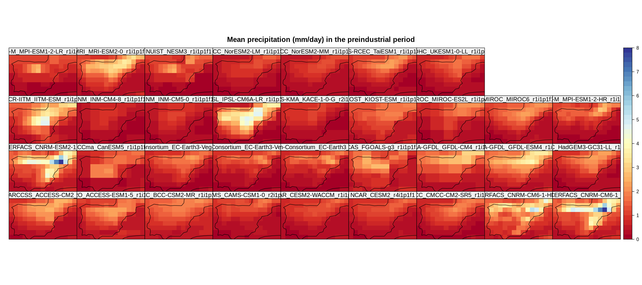
Before we continue we can take a look at the data by, for instance, plotting maps. To do so we first compute the climatology with function climatology from the transformeR package. Finally, we use the spatialPlot function from the visualizeR package (run help(spatialPlot) to check different plotting parameters).
cmip6.hist.c <- climatology(cmip6.hist)
spatialPlot(cmip6.hist.c,
            backdrop.theme = "coastline",
            col.theme = "Blues",
            at = seq(0, 8, 0.2),
            set.max = 8, set.min = 0,
            layout = c(9, 4),
            main = "Mean precipitation (mm/day) in the preindustrial period",
            strip = strip.custom(factor.levels = cmip6.hist.c$Members))
[2024-11-08 10:59:57.7728] - Computing climatology...

[2024-11-08 10:59:57.827338] - Done.
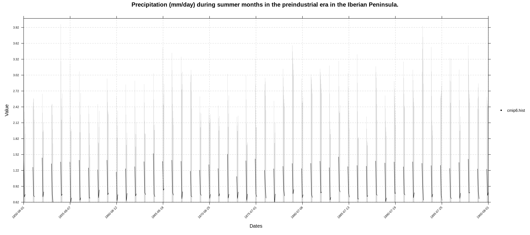
We could also display the temporal series with temporalPlot for the original monthly values…
temporalPlot(cmip6.hist, xyplot.custom = list(main = "Precipitation (mm/day) during summer months in the preindustrial era in the Iberian Peninsula."))
pad applied on the interval: month
…or the aggregated yearly values by previously applying the aggregateGrid function (we will change the color this time, run help(temporalPlot) for further customization):
cmip6.hist.y <- aggregateGrid(cmip6.hist, aggr.y = list(FUN = "mean", na.rm = T))
temporalPlot(cmip6.hist.y,
             cols = "orange",
             xyplot.custom = list(main = "Summer mean precipitation (mm/day) in the preindustrial era in the Iberian Peninsula."))
[2024-11-08 11:00:02.105277] Performing annual aggregation...

[2024-11-08 11:00:03.369865] Done.

pad applied on the interval: year
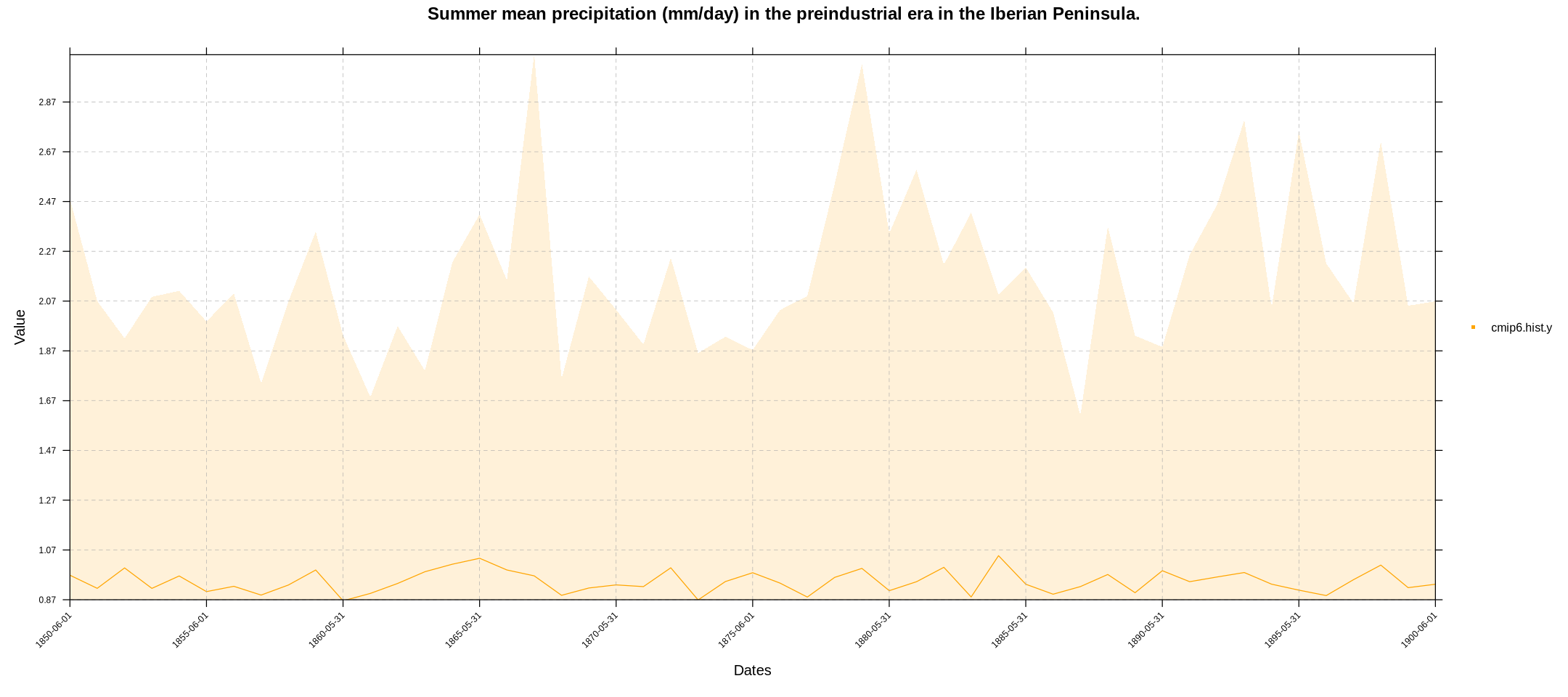
Note that the temporalPlot function recognizes that our grid is multi-member (multi-model in this case) and shows the ensemble mean (solid line) and the multi-member spread (shadow).
3.5. Calculation of anomalies (future projections - historical simulations)#
We will now calculate the relative precipitation anomaly of a fixed future period (e.g. 2041-2060) relative to the preindustrial period. We will consider the SSP585 mitigation scenario. Therefore, we now point to another data source:
data.file.ssp585 <- subset(df, project == "CMIP6" & variable == "pr" & experiment == "ssp585" & type == "opendap")[["location"]]
cmip6.fut <- loadGridData(data.file.ssp585,
             var = "pr",
             lonLim = c(-10, 4), latLim = c(36, 44),
             season = 6:8,
             years = 2041:2060)
[2024-11-08 11:00:03.758623] Opening dataset...

[2024-11-08 11:00:04.096763] The dataset was successfuly opened

[2024-11-08 11:00:04.10151] Defining geo-location parameters

[2024-11-08 11:00:04.165869] Defining time selection parameters

[2024-11-08 11:00:04.185969] Retrieving data subset ...

[2024-11-08 11:00:09.657921] Done
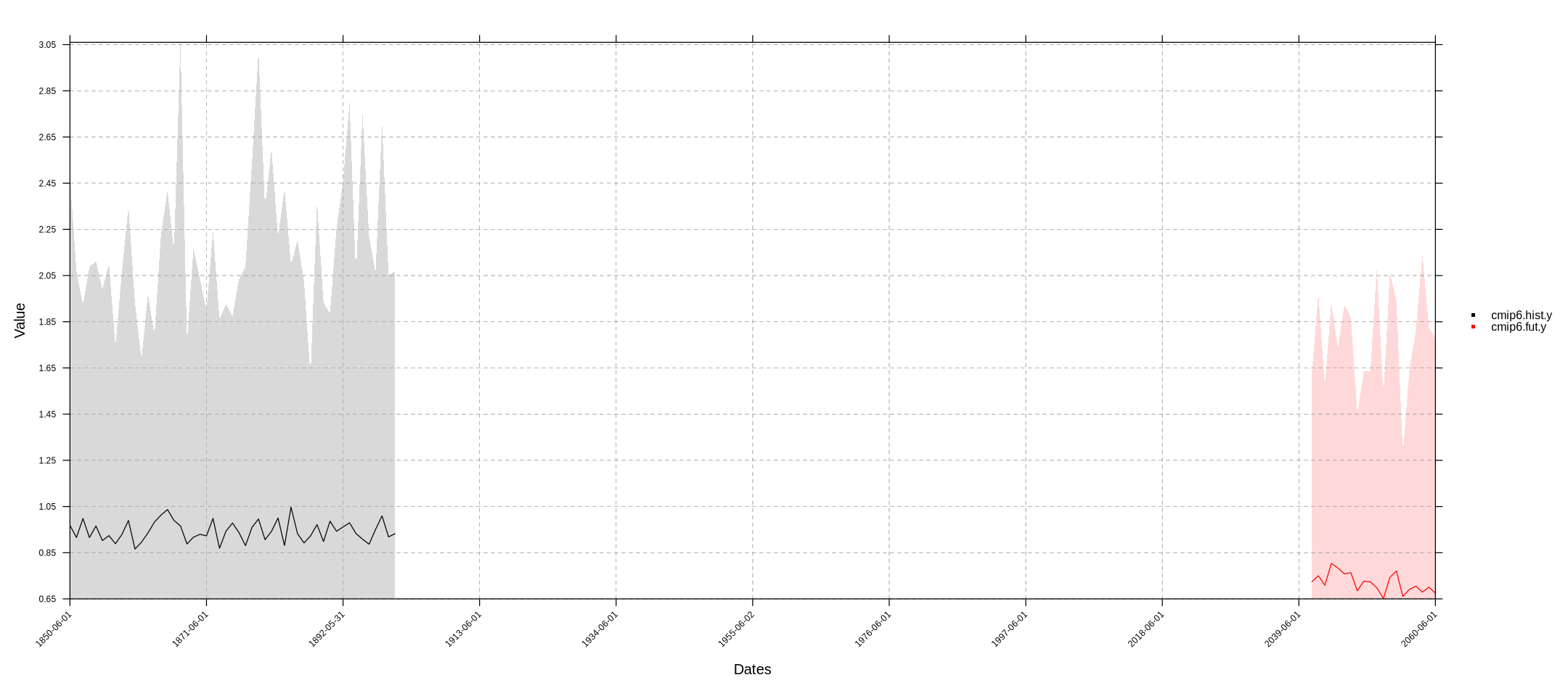
We can combine the output with the historical data in the same time-series plot:
cmip6.fut.y <- aggregateGrid(cmip6.fut, aggr.y = list(FUN = "mean", na.rm = T))
temporalPlot(cmip6.hist.y, cmip6.fut.y)
[2024-11-08 11:00:09.676278] Performing annual aggregation...

[2024-11-08 11:00:10.236048] Done.

pad applied on the interval: year

pad applied on the interval: year
Lets calculate the anomaly. To do so, we must retain the common available members in both grids. These are de members (CMIP6 models) in the historical period:
cmip6.hist$Members
- 'CSIRO-ARCCSS_ACCESS-CM2_r1i1p1f1'
- 'CSIRO_ACCESS-ESM1-5_r1i1p1f1'
- 'BCC_BCC-CSM2-MR_r1i1p1f1'
- 'CAMS_CAMS-CSM1-0_r2i1p1f1'
- 'NCAR_CESM2-WACCM_r1i1p1f1'
- 'NCAR_CESM2_r4i1p1f1'
- 'CMCC_CMCC-CM2-SR5_r1i1p1f1'
- 'CNRM-CERFACS_CNRM-CM6-1-HR_r1i1p1f2'
- 'CNRM-CERFACS_CNRM-CM6-1_r1i1p1f2'
- 'CNRM-CERFACS_CNRM-ESM2-1_r1i1p1f2'
- 'CCCma_CanESM5_r1i1p1f1'
- 'EC-Earth-Consortium_EC-Earth3-Veg-LR_r1i1p1f1'
- 'EC-Earth-Consortium_EC-Earth3-Veg_r1i1p1f1'
- 'EC-Earth-Consortium_EC-Earth3_r1i1p1f1'
- 'CAS_FGOALS-g3_r1i1p1f1'
- 'NOAA-GFDL_GFDL-CM4_r1i1p1f1'
- 'NOAA-GFDL_GFDL-ESM4_r1i1p1f1'
- 'MOHC_HadGEM3-GC31-LL_r1i1p1f3'
- 'CCCR-IITM_IITM-ESM_r1i1p1f1'
- 'INM_INM-CM4-8_r1i1p1f1'
- 'INM_INM-CM5-0_r1i1p1f1'
- 'IPSL_IPSL-CM6A-LR_r1i1p1f1'
- 'NIMS-KMA_KACE-1-0-G_r2i1p1f1'
- 'KIOST_KIOST-ESM_r1i1p1f1'
- 'MIROC_MIROC-ES2L_r1i1p1f2'
- 'MIROC_MIROC6_r1i1p1f1'
- 'MPI-M_MPI-ESM1-2-HR_r1i1p1f1'
- 'MPI-M_MPI-ESM1-2-LR_r1i1p1f1'
- 'MRI_MRI-ESM2-0_r1i1p1f1'
- 'NUIST_NESM3_r1i1p1f1'
- 'NCC_NorESM2-LM_r1i1p1f1'
- 'NCC_NorESM2-MM_r1i1p1f1'
- 'AS-RCEC_TaiESM1_r1i1p1f1'
- 'MOHC_UKESM1-0-LL_r1i1p1f2'
and these in the future period for the SSP585 scenario:
cmip6.fut$Members
- 'CSIRO-ARCCSS_ACCESS-CM2_r1i1p1f1'
- 'CSIRO_ACCESS-ESM1-5_r1i1p1f1'
- 'BCC_BCC-CSM2-MR_r1i1p1f1'
- 'CAMS_CAMS-CSM1-0_r2i1p1f1'
- 'NCAR_CESM2-WACCM_r1i1p1f1'
- 'NCAR_CESM2_r4i1p1f1'
- 'CMCC_CMCC-CM2-SR5_r1i1p1f1'
- 'CNRM-CERFACS_CNRM-CM6-1-HR_r1i1p1f2'
- 'CNRM-CERFACS_CNRM-CM6-1_r1i1p1f2'
- 'CNRM-CERFACS_CNRM-ESM2-1_r1i1p1f2'
- 'CCCma_CanESM5_r1i1p1f1'
- 'EC-Earth-Consortium_EC-Earth3-Veg_r1i1p1f1'
- 'EC-Earth-Consortium_EC-Earth3_r1i1p1f1'
- 'CAS_FGOALS-g3_r1i1p1f1'
- 'NOAA-GFDL_GFDL-CM4_r1i1p1f1'
- 'NOAA-GFDL_GFDL-ESM4_r1i1p1f1'
- 'MOHC_HadGEM3-GC31-LL_r1i1p1f3'
- 'CCCR-IITM_IITM-ESM_r1i1p1f1'
- 'INM_INM-CM4-8_r1i1p1f1'
- 'INM_INM-CM5-0_r1i1p1f1'
- 'IPSL_IPSL-CM6A-LR_r1i1p1f1'
- 'NIMS-KMA_KACE-1-0-G_r2i1p1f1'
- 'KIOST_KIOST-ESM_r1i1p1f1'
- 'MIROC_MIROC-ES2L_r1i1p1f2'
- 'MIROC_MIROC6_r1i1p1f1'
- 'MPI-M_MPI-ESM1-2-HR_r1i1p1f1'
- 'MPI-M_MPI-ESM1-2-LR_r1i1p1f1'
- 'MRI_MRI-ESM2-0_r1i1p1f1'
- 'NUIST_NESM3_r1i1p1f1'
- 'NCC_NorESM2-LM_r1i1p1f1'
- 'NCC_NorESM2-MM_r1i1p1f1'
- 'AS-RCEC_TaiESM1_r1i1p1f1'
- 'MOHC_UKESM1-0-LL_r1i1p1f2'
As is the case in this example, different scenarios for different variables may have less members than the corresponding historical experiment. We can therefore subset the historical grid to match the members with the future grid. An easy way to retain the common members in both grids is to use the function intersectGrid (which also allows for spatial and temporal intersections, by changing the value in the type argument):
cmip6.common.mems <- intersectGrid(cmip6.hist, cmip6.fut, type = "members", which.return = 1:2)
cmip6.hist.s <- cmip6.common.mems[[1]] ; cmip6.fut <- cmip6.common.mems[[2]]
It is always a good practice to make sure that the members in both grids are identical:
identical(cmip6.hist.s$Members, cmip6.fut$Members)
Now we can calculate the anomaly by computing the difference between both climatologies:
anom <- gridArithmetics(climatology(cmip6.fut), climatology(cmip6.hist.s), operator = "-")
[2024-11-08 11:00:10.526133] - Computing climatology...

[2024-11-08 11:00:10.706641] - Done.

[2024-11-08 11:00:10.71262] - Computing climatology...

[2024-11-08 11:00:10.745056] - Done.
We can calculate the relative anomaly the same way:
rel.anom <- gridArithmetics(anom, climatology(cmip6.hist.s), 100, operator = c("/", "*"))
[2024-11-08 11:00:10.766294] - Computing climatology...

[2024-11-08 11:00:10.805385] - Done.
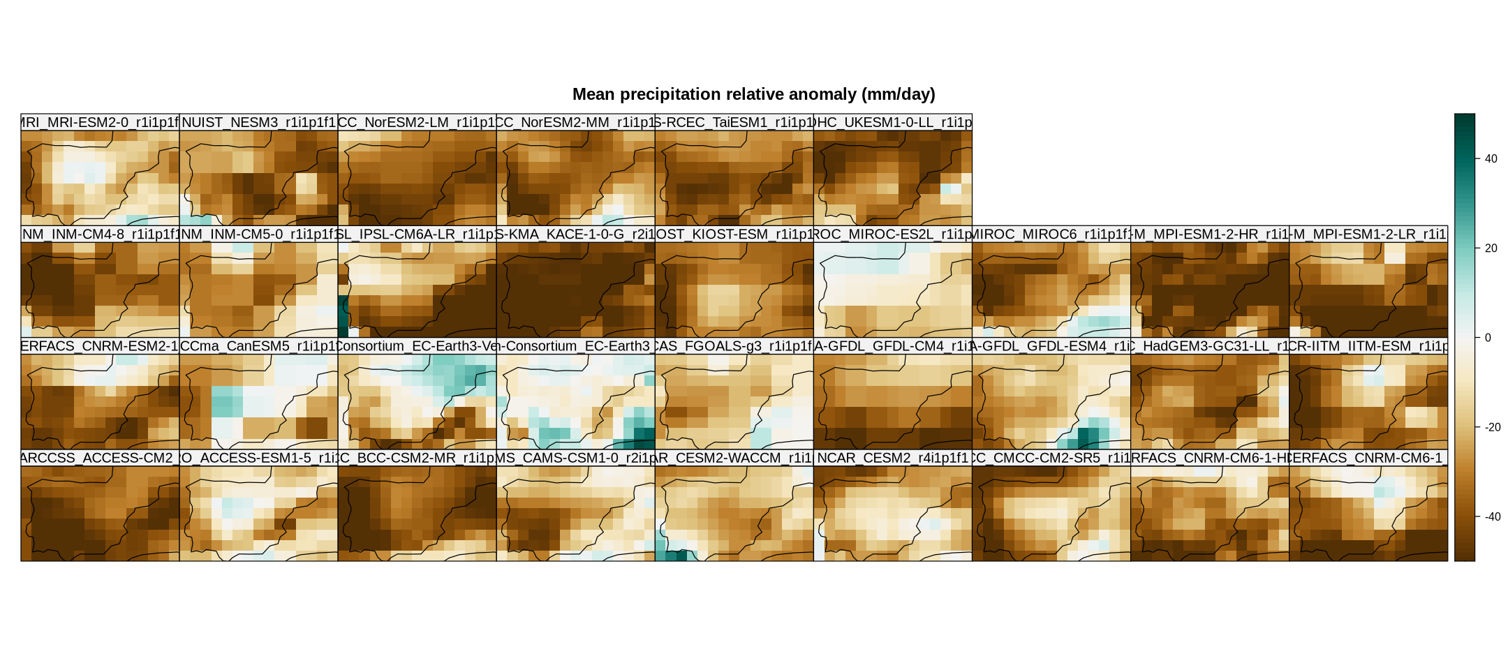
Finally, we can plot the output using an appropriate palette for the color.theme:
spatialPlot(rel.anom,
            color.theme = "BrBG",
            backdrop.theme = "coastline",
            at = seq(-50, 50),
            set.max = 50, set.min = -50,
            layout = c(9, 4),
            main = "Mean precipitation relative anomaly (mm/day)",
            strip = strip.custom(factor.levels = cmip6.fut$Members))
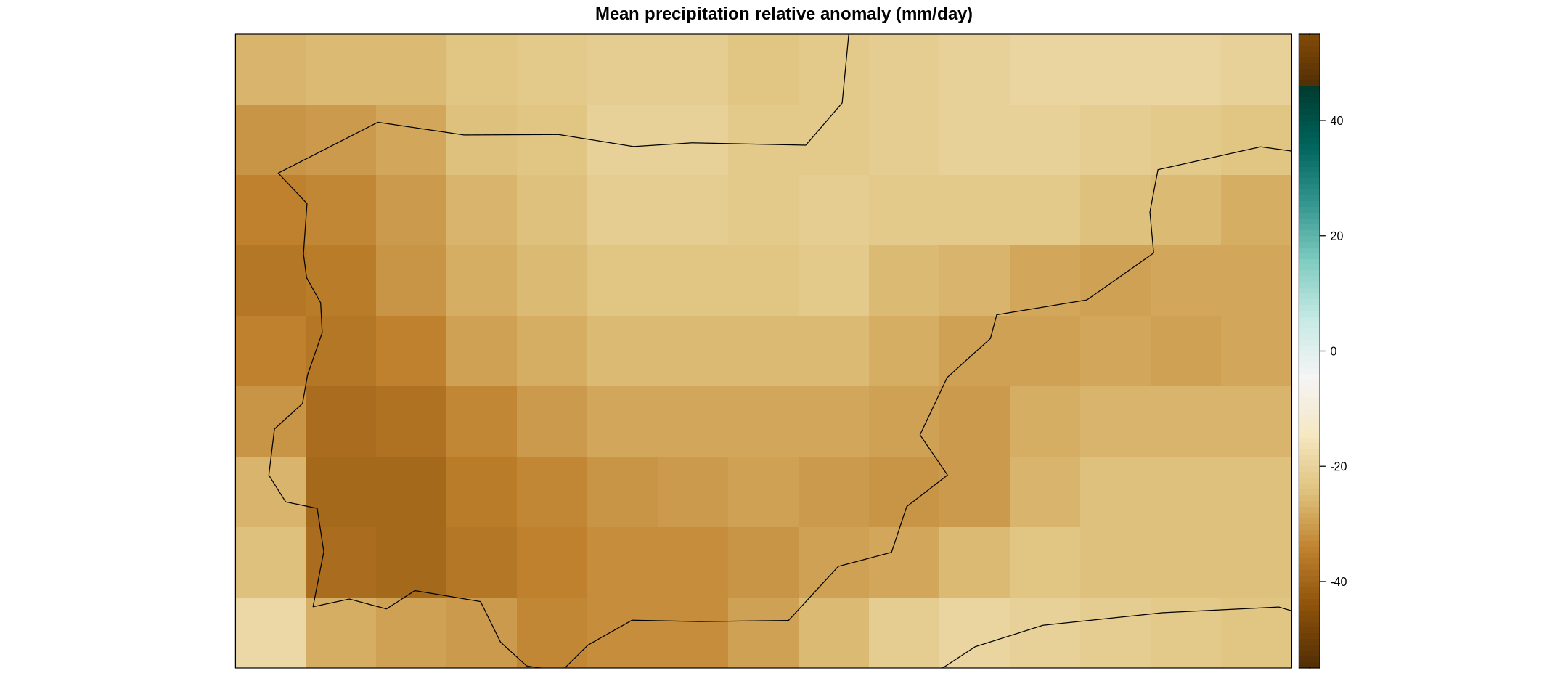
We can do the same for the multi-model ensemble mean by previously applying the aggregateGrid function:
ens.mean.anom <- aggregateGrid(rel.anom, aggr.mem = list(FUN = "mean", na.rm = TRUE))
spatialPlot(ens.mean.anom,
            color.theme = "BrBG",
            backdrop.theme = "coastline",
            at = seq(-55, 55),
            set.max = 55, set.min = -55,
            main = "Mean precipitation relative anomaly (mm/day)",
            strip = strip.custom(factor.levels = cmip6.fut$Members))
[2024-11-08 11:00:14.246094] - Aggregating members...

[2024-11-08 11:00:14.248896] - Done.
3.6. Spatial aggregation#
The time series plots we have created above, automatically performs spatial aggregations. However, we can control this operation by using the aggr.spatial parameter in the aggregateGrid function, which by default calculates weighted values according to the latitude. If we aggregate the rel.anom object, we will get a single value per model (member).
rel.anom.regional_mean <- aggregateGrid(rel.anom, aggr.spatial = list(FUN = "mean", na.rm = TRUE))
Calculating areal weights...

[2024-11-08 11:00:14.441585] - Aggregating spatially...

[2024-11-08 11:00:14.443421] - Done.
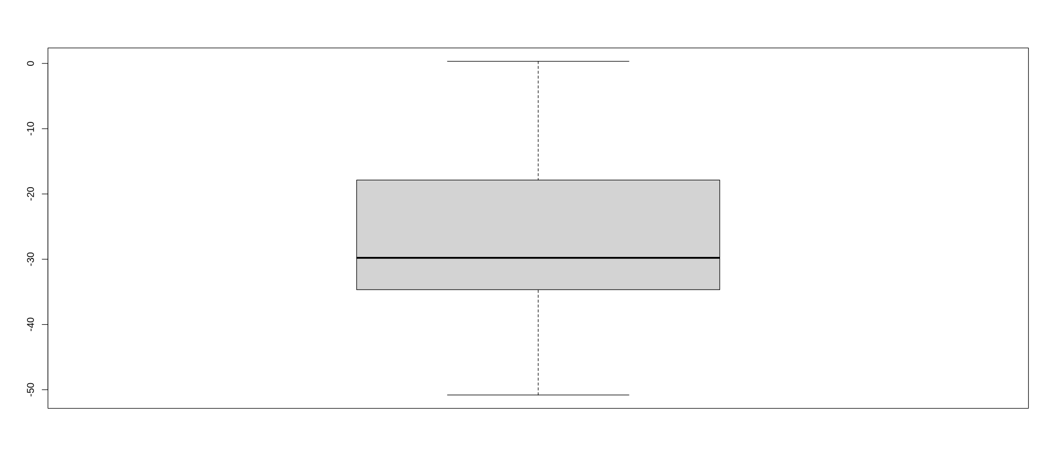
In the next code chunk we get the multi-model mean and the percentiles:
m <- aggregateGrid(rel.anom.regional_mean, aggr.mem = list(FUN = "mean", na.rm = TRUE))
p25 <- aggregateGrid(rel.anom.regional_mean, aggr.mem = list(FUN = "quantile", prob = 0.25, na.rm = TRUE))
p75 <- aggregateGrid(rel.anom.regional_mean, aggr.mem = list(FUN = "quantile", prob = 0.75, na.rm = TRUE))

c("mean" = m$Data, "P25" = p25$Data, "P75" = p75$Data)
[2024-11-08 11:00:14.456018] - Aggregating members...

[2024-11-08 11:00:14.457539] - Done.

[2024-11-08 11:00:14.459882] - Aggregating members...

[2024-11-08 11:00:14.462046] - Done.

[2024-11-08 11:00:14.464226] - Aggregating members...

[2024-11-08 11:00:14.466114] - Done.
- mean
- -27.2475711759013
- P25
- -34.6696350110102
- P75
- -17.8717848503489
At this stage it is easy to operate directly with the data array and use other R functionalities, for instance:
boxplot(rel.anom.regional_mean$Data)
The climate4R framework provides many other spatial and temporal operations functionalities, such as interpolation, subsetting or spatial intersection. It also provides functionalities for bias correction and downscaling (see Iturbide et al., 2019. DOI: 10.1016/j.envsoft.2018.09.009).
Session Info#
sessionInfo()
R version 4.3.3 (2024-02-29)
Platform: x86_64-conda-linux-gnu (64-bit)
Running under: Ubuntu 22.04.5 LTS

Matrix products: default
BLAS/LAPACK: /home/zequi/miniconda3/lib/libopenblasp-r0.3.21.so;  LAPACK version 3.9.0

locale:
 [1] LC_CTYPE=en_US.UTF-8          LC_NUMERIC=C
 [3] LC_TIME=es_ES.UTF-8           LC_COLLATE=en_US.UTF-8
 [5] LC_MONETARY=es_ES.UTF-8       LC_MESSAGES=en_US.UTF-8
 [7] LC_PAPER=es_ES.UTF-8          LC_NAME=es_ES.UTF-8
 [9] LC_ADDRESS=es_ES.UTF-8        LC_TELEPHONE=es_ES.UTF-8
[11] LC_MEASUREMENT=es_ES.UTF-8    LC_IDENTIFICATION=es_ES.UTF-8

time zone: Europe/Madrid
tzcode source: system (glibc)

attached base packages:
[1] stats     graphics  grDevices utils     datasets  methods   base

other attached packages:
[1] magrittr_2.0.3      lattice_0.22-6      visualizeR_1.6.4
[4] transformeR_2.2.2   loadeR_1.8.2        climate4R.UDG_0.2.6
[7] loadeR.java_1.1.1   rJava_1.0-11        repr_1.1.7

loaded via a namespace (and not attached):
 [1] dotCall64_1.1-1         spam_2.10-0             latticeExtra_0.6-30
 [4] vctrs_0.6.5             mapplots_1.5.2          tools_4.3.3
 [7] bitops_1.0-8            generics_0.1.3          parallel_4.3.3
[10] tibble_3.2.1            proxy_0.4-27            fansi_1.0.6
[13] SpecsVerification_0.5-3 pkgconfig_2.0.3         data.table_1.15.2
[16] RColorBrewer_1.1-3      uuid_1.2-1              lifecycle_1.0.4
[19] compiler_4.3.3          kohonen_3.0.12          deldir_2.0-4
[22] fields_16.2             munsell_0.5.1           akima_0.6-3.4
[25] htmltools_0.5.8.1       maps_3.4.2              RCurl_1.98-1.13
[28] pillar_1.9.0            crayon_1.5.3            MASS_7.3-60.0.1
[31] boot_1.3-31             abind_1.4-5             vioplot_0.5.0
[34] padr_0.6.2              verification_1.42       tidyselect_1.2.1
[37] digest_0.6.37           dplyr_1.1.4             fastmap_1.2.0
[40] grid_4.3.3              colorspace_2.1-1        cli_3.6.3
[43] base64enc_0.1-3         utf8_1.2.4              sm_2.2-6.0
[46] IRdisplay_1.1           withr_3.0.1             scales_1.3.0
[49] sp_2.1-4                IRkernel_1.3.2          jpeg_0.1-10
[52] interp_1.1-6            pbdZMQ_0.3-10           RcppEigen_0.3.4.0.1
[55] zoo_1.8-12              png_0.1-8               pbapply_1.7-2
[58] evaluate_1.0.0          dtw_1.23-1              viridisLite_0.4.2
[61] rlang_1.1.4             Rcpp_1.0.13             glue_1.7.0
[64] easyVerification_0.4.5  CircStats_0.2-6         jsonlite_1.8.9
[67] R6_2.5.1